Information
Title: Progressive Distillation for Fast Sampling of Diffusion Models (ICLR 2022)
Reference
Author: Sangwoo Jo
Last updated on Nov. 14, 2023
Progressive Distillation for Fast Sampling of Diffusion Models#
1. Introduction#
Diffusion model 이 ImageNet generation task 에서 기존 BigGAN-deep 그리고 VQ-VAE-2 모델보다 FID/CAS score 기준으로 더 좋은 성능을 보여주며 많은 각광을 받고 있습니다. 그러나 sampling 속도가 느리다는 치명적인 단점을 가지고 있습니다.
이를 해결하기 위해, 논문에서는 Progressive Distillation 기법을 소개하게 됩니다. 간략히 설명하자면 사전학습된 \(N\)-step DDIM 모델을 \(N/2\)-step student 모델에 distillation 하는 과정을 반복하여 최종적으로 4 steps 만으로도 state-of-the-art 모델을 수천번의 sampling steps 를 거쳐 생성한 이미지들과 유사한 모델 성능을 보여준다고 합니다.
2. Background - Diffusion model in continuous time#
2.1. Definition#
Continuous 한 time domain 에서의 diffusion model 을 다음과 같은 요소들로 정의합니다.
Training data \(x \sim p(x)\)
Latent variables \(z = \{z_t | t \in [0,1]\}\)
여기서 \(z_t\) 는 differentiable 한 noise schedule functions \(\alpha_t, \sigma_t\) 로 값이 정의되고, 이 함수들은 log signal-to-noise-ratio \(\lambda_t = \log[\alpha_t^2/\sigma_t^2]\) 가 monotonically decreasing 하도록 설정됩니다. 그리고 이들을 기반으로 다음과 같은 Markovian forward process 를 정의합니다.

Fig. 400 Markovian Forward Process#
where \(0 \leq s < t \leq 1\) and \(\sigma_{t|s}^2 = (1-e^{\lambda_t - \lambda_s}) \sigma_t^2\)
2.2. Objective#
Diffusion model 의 objective 는 \(\hat{x}_{\theta}(z_t)\) 모델에서 \(z_t \sim q(z_t | x)\) 와 \(\lambda_t\) 를 입력받아 다음과 같이 Mean Squared Error Loss 를 최소화하는 방향으로 원본 이미지 \(x\) 를 예측하는 것입니다. 이때, \(w(\lambda_t)\) 를 weighting function 이라 부릅니다.
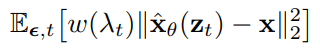
Fig. 401 Objective#
where \(t \sim U[0,1]\)
2.3. Sampling#
Diffusion model 에서 sampling 하는 방식은 다양하게 존재합니다.
2.3.1. Ancestral Sampling - DDPM#
첫번째로는 DDPM 논문에서 소개하는 discrete time ancestral sampling 방식입니다. 위에 소개했던 notation 기준으로 reverse process 를 다음과 같이 수식적으로 표현 가능합니다.

Fig. 402 Reverse Process#
이를 기반으로 \(z_1 \sim N(0,I)\) 로부터 다음과 같은 ancestral sampler 를 정의하게 됩니다. 이때, \(\gamma\) 는 sampling 시 얼마나 많은 noise 를 추가할지 설정하는 hyperparameter 입니다.
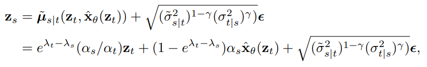
Fig. 403 Ancestral Sampler#
2.3.2. Probability Flow ODE#
반면에, Song et al. (2021c) 에서 forward diffusion process 를 SDE 로 표현할 수 있고, 이를 통한 sampling process 를 probabiility flow ODE 로 표현해서 구할 수 있다고 제시합니다.
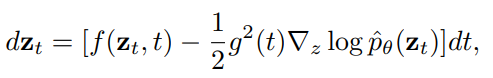
Fig. 404 Probability flow ODE#
이때, \(f(z_t,t) = \frac{d \log \alpha_t}{dt}z_t, g^2(t) = \frac{dσ_t^2}{dt} − 2 \frac{d\log \alpha_t}{dt}\sigma_t^2, \text{and}\) \(\nabla_z \log \hat{p}_{\theta}(z_t) = \frac{\alpha_t\hat{x}_{\theta}(z_t) -z_t}{\sigma_t^2}\) 로 정의합니다.
다시 말해 \(z_1 \sim N(0,I)\) 로부터 이미지 \(x\) 를 생성하는 task 를 위와 같이 ODE solver 문제로 해석할 수 있고, Euler rule 이나 Runge-Kutta method 등의 전통적인 ODE integrator 보다 DDIM sampler 를 적용했을때 성능이 가장 좋다고 논문에서 제시합니다. 아래 사진은 다양한 Probabiltity Flow ODE solver 들의 128x128 ImageNet 데이터셋 FID 성능을 비교한 결과입니다.
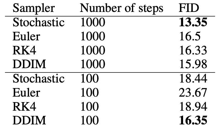
Fig. 405 FID scores on 128 × 128 ImageNet for various probability flow ODE integrators#
참고로 DDIM sampler 를 ODE solver 문제로 해석하면 다음과 같이 표현할 수 있고, 이 수식은 앞으로 자주 보게 될 예정입니다.
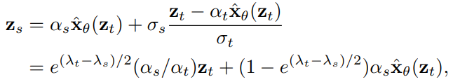
Fig. 406 DDIM sampler#
3. Progressive Distillation#
Diffusion model 을 더 효율적으로 sampling 하기 위해 소개한 progressive distillation 기법은 다음과 같은 절차로 진행됩니다.
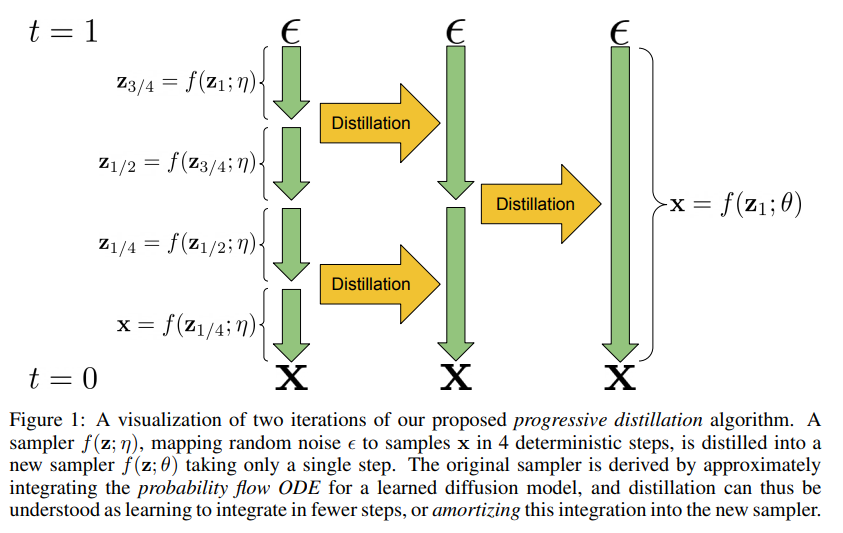
Fig. 407 Progressive Distillation#
Standard diffusion training 기법으로 Teacher Diffusion Model 학습
Student Model 정의 - Teacher Model 로부터 모델 구조 및 parameter 복사
Student Model 학습
이때, original data \(x\) 대신에 \(\tilde{x}\) 를 target 로 student model 을 학습합니다. \(\tilde{x}\) 에 대한 공식은 아래 pseudocode 에 소개되는데, 이는 one-step student sample \(\tilde{z}_{t''}\) 과 two-step teacher sample \(z_{t''}\) 를 일치시키기 위해 나온 공식입니다.
2 DDIM steps of teacher model 결과와 1 DDIM step of student model 결과를 일치시키는 것이 핵심입니다. 여기서 \(z_t\) 에서 \(z_{t-1/N}\) 로 넘어가는 과정을 1 DDIM step 라 정의하고, \(N\) 은 총 진행되는 student sampling steps 입니다.
기존 denoising model 학습 시, \(x\) 가 \(z_t\) 에 대해 deterministic 하지 않기 때문에 (다른 \(x\) 값들에 대해 동일한 \(z_t\) 생성 가능) 모델은 사실상 \(x\) 가 아닌 weighted average of possible \(x\) values 를 예측하는 모델이라고 합니다. 따라서, \(z_t\)에 대해 deterministic 한 \(\tilde{x}(z_t)\) 를 예측하도록 학습한 student model 은 teacher model 보다 더 sharp 한 prediction 을 할 수 있다고 주장합니다.
Student Model 이 새로운 Teacher Model 이 되고 sampling steps \(N\) → \(N/2\) 로 줄어드는 이 과정을 계속 반복
이에 대한 pseudocode 도 확인해보겠습니다.
PseudoCode
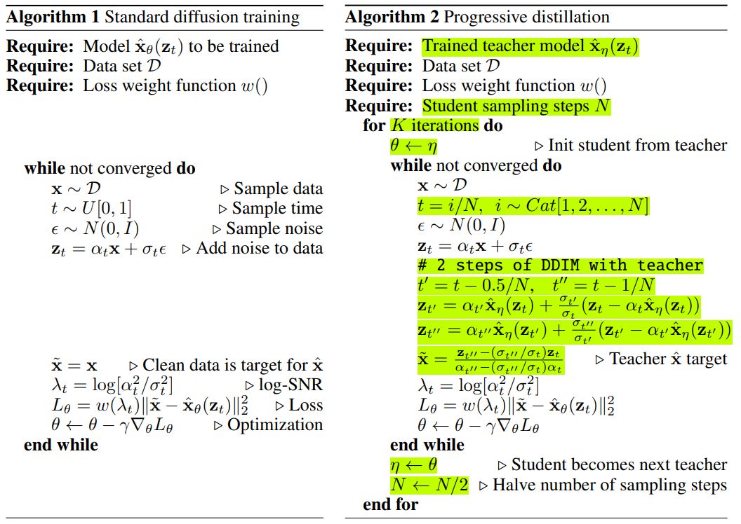
Fig. 408 Pseudocode for Progresssive Distillation#
4. Diffusion Model Parameterization and Training Loss#
이제 denoising model \(\hat{x}_{\theta}\) 와 reconstruction loss weight \(w(\lambda_t)\) 에 대한 설정값에 대해 자세히 알아보겠습니다. 우선, 논문에서는 일반성을 잃지 않고 (without loss of generalization) variance-preserving diffusion process (i.e., \(\alpha_t^2 + \sigma_t^2 = 1\) ) 라는 가정을 하게 됩니다. 더 자세하게는 cosine schedule \(\alpha_t = cos(0.5\pi t)\) 를 사용합니다.
DDPM 을 비롯한 대다수의 논문에서 이미지 \(x\) 가 아닌 noise \(\epsilon\) 를 예측하는 denoising model \(\hat{\epsilon}_{\theta}(z_t)\) 를 정의합니다. \(\epsilon\)-space 에 정의된 손실함수에 \(\hat{x_{\theta}}(z_t) = \frac{1}{\alpha_t}(z_t - \sigma_t \hat{\epsilon}_{\theta}(z_t))\) 식을 대입해보겠습니다.

Fig. 409 Training loss on \(\epsilon\)-space and \(x\)-space#
따라서, 이는 이미지 \(x\) domain 에서 weighted reconstruction loss 를 적용하는 것과 동일하며 이때 weighting function \(w(\lambda_t) = exp(\lambda_t), \lambda_t = \log[\alpha_t^2/\sigma_t^2]\) 로 정의할 수 있습니다. 그러나 이러한 standard training procedure 는 progressive distillation 에 적합하지 않다고 주장합니다.
Standard diffusion training 기법에서는 다양한 범위 내에서의 signal-to-noise ratio \(\alpha_t^2/\sigma_t^2\) 에서 모델이 학습되지만, distillation 이 진행될수록 이 signal-to-noise ratio 가 감소한다는 단점을 확인하게 됩니다. 더 자세히 설명하자면, \(t\) 가 증가할수록 signal-to-noise-ratio \(\alpha_t^2/\sigma_t^2\) 는 0 에 가까워지게 되고, \(\hat{x_{\theta}}(z_t) = \frac{1}{\alpha_t}(z_t - \sigma_t \hat{\epsilon}_{\theta}(z_t))\) 에서 \(\alpha_t \rightarrow 0\) 이므로 \(\hat{\epsilon}_{\theta}(z_t)\) 에 대한 \(x\)-prediction 변화량이 점차적으로 커지게 됩니다. 이는 여러번의 training step 을 거칠 때 상관없지만, sampling steps 가 줄어들수록 치명적이게 됩니다. 최종적으로 sampling steps=1 일 때까지 progressively distillation 을 적용하면 모델의 입력으로는 단순한 pure noise \(\epsilon\) (i.e., \(\alpha_t = 0, \sigma_t = 1\) ) 이 들어가게 되고, \(\epsilon\)-prediction 과 \(x\)-prediction 의 상관관계가 완전히 사라지게 됩니다. 이는 위 loss function 에서 weighting function \(w(\lambda_t) = 0\) 인 부분에서 확인할 수 있습니다.
그래서 논문에서는 다음과 같은 세가지 방법으로 stable 한 \(\hat{x}_{\theta}(z_t)\) prediction 을 구할 수 있는 방법들을 제시합니다.
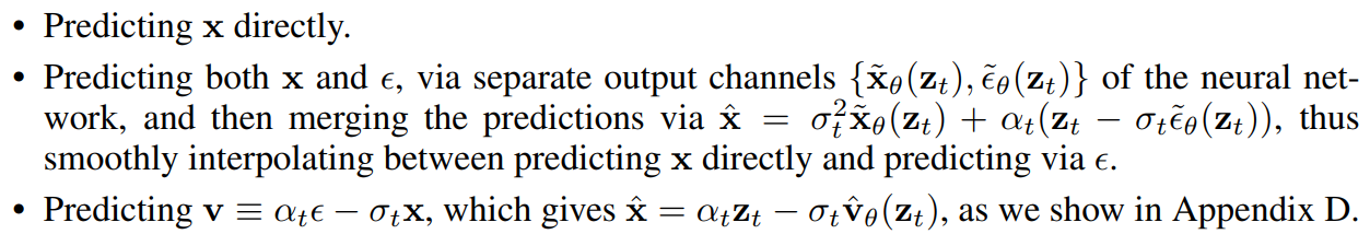
Fig. 410 Different parameterizations#
Weighting function \(w(\lambda_t)\) 도 두 가지 방안으로 실험했습니다. 이는 signal-to-noise ratio 가 0 으로 수렴하는 현상을 방지하도록 설정되었다고 합니다.
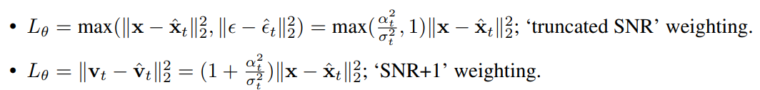
Fig. 411 Different loss weighting functions#
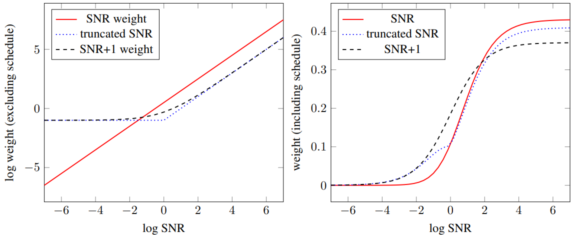
Fig. 412 Visualization of different loss weighting functions#
5. Experiments#
논문에서 32x32 부터 128x128 까지 다양한 resolution 에서 모델 성능을 확인했습니다. 또한, cosine schedule \(\alpha_t = cos(0.5 \pi t)\) 그리고 DDPM 에서 소개한 U-Net 아키텍쳐를 사용했으며 부가적으로 Nichol & Dhariwal (2021), Song et al. (2021c) 에서 사용된 BigGAN-style up/downsampling 기법을 활용했습니다.
5.1. Model Parametrization and Training Loss#
아래 지표는 unconditional CIFAR-10 데이터셋에 앞써 소개드린 \(\epsilon\)-prediction 외에 다른 세 가지 parametrization 기법들로 original diffusion model 의 FID 와 Inception Score 성능을 확인해본 결과입니다.
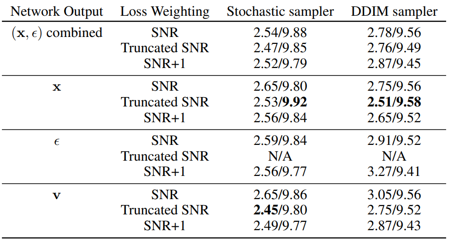
Fig. 413 Ablation Study on Parameterizations and Loss Weightings#
성능을 비교해본 결과 \(v\)-prediction/\(x\)-prediction 과 Truncated SNR loss function 을 사용했을때 성능이 가장 좋은 부분을 확인할 수 있습니다. 또한, \(\epsilon\)-prediction 과 Truncated SNR loss function 의 조합을 사용하여 학습 시, unstable 한 convergence 를 보이는 현상도 볼 수 있습니다.
위 실험결과를 바탕으로 progressive distillation 진행시 CIFAR-10 데이터셋에는 \(x\)-prediction, 그 외 데이터셋에서는 \((x,\epsilon)\)-prediction 을 사용했다고 합니다. 더 자세한 hyperparameter setting 은 Appendix E 참조하시면 됩니다.
5.2. Progressive Distillation#
논문에서 CIFAR-10, 64x64 downsampled ImageNet, 128 × 128 LSUN bedrooms, 그리고 128 × 128 LSUN Church-Outdoor 데이터셋에 progressive distillation 을 적용하여 모델 성능을 측정합니다. CIFAR-10 데이터셋 기준으로 teacher model 로부터 progressive distillation 진행 시 8192 steps 부터 시작하였고 batch size=128 로 설정하였습니다. 그 외 resolution 이 큰 데이터셋에 대해서는 1024 steps 부터 시작하고 batch size=2048 로 실험을 진행했습니다. 또한, 매 iteration 마다 \(10^{-4}\) 에서 \(0\) 으로 learning rate 를 linearly anneal 했다고 합니다.
FID 성능을 확인해본 결과, 실험을 진행한 모든 4개의 데이터셋에 대해 progressive distillation 을 통해 4-8 sampling steps 만 진행해도 undistilled DDIM 그리고 stochastic sampler 에 준하는 성능을 보여주는 것을 확인할 수 있습니다. 4 sampling steps 까지 progressive distillation 진행하면서 발생하는 computational cost 가 baseline 모델 학습하는 것과 비슷한 부분을 생각했을때 엄청난 장점이라고 생각합니다.
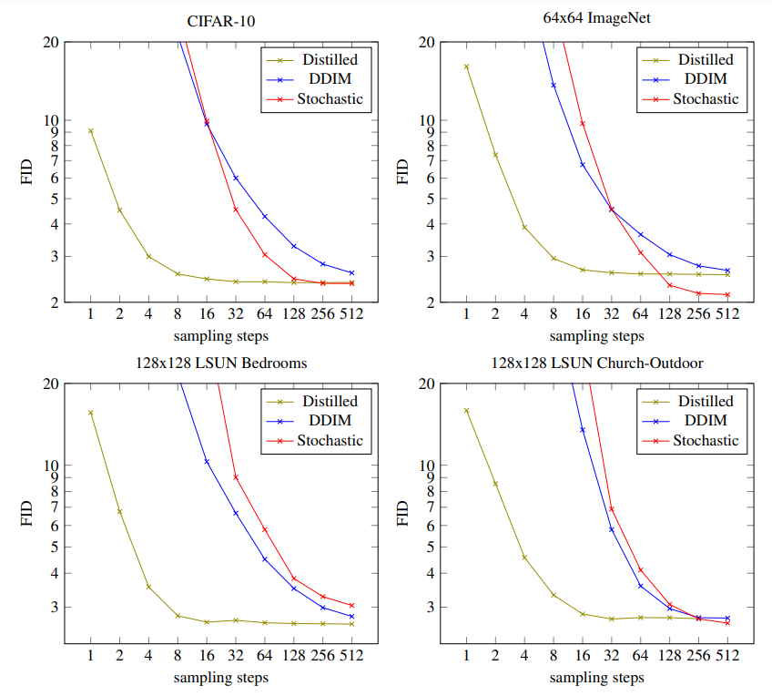
Fig. 414 Comparison between Distilled, DDIM, and Stochastic Sampler#
추가적으로 CIFAR-10 데이터셋에서 타 fast sampling method 들과 FID 성능을 비교해본 결과입니다.
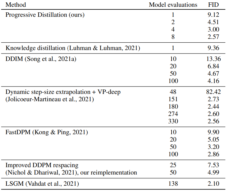
Fig. 415 Comparison of fast sampling results#
그리고 64x64 ImageNet 데이터셋에 distilled 모델로 생성한 예시 이미지들입니다. 동일한 seed 에 대해서 input noise 로부터 output image 까지 mapping 이 잘되는 부분을 확인할 수 있습니다.
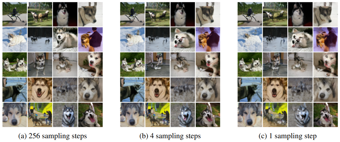
Fig. 416 Random samples from distilled 64 × 64 ImageNet models#
마지막으로 distillation scheduling 에 대한 ablation study 도 논문에서 진행했습니다. 첫번째 ablation study 로는 매 distillation iteration 마다 parameter update 횟수를 \(50k\) 에서 \(25k, 10k, 5k\) 로 점차 줄이면서 FID 성능을 비교해보고, 두번째 ablation study 로는 매 distillation iteration 마다 sampling step 을 2배 대신에 4배씩 줄여가면서 student model 을 학습하여 성능을 비교합니다. 그 결과 parameter update 횟수를 현저히 줄임에도 불구하고 FID 성능이 크게 줄지 않는 반면, 각 iteration 마다 sampling step 을 4배씩 줄이는 학습방식으로는 모델 성능이 좋지 못한 부분을 확인할 수 있습니다.
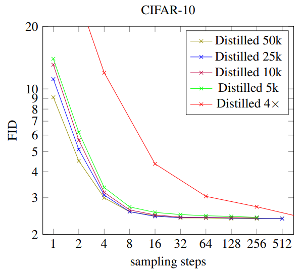
Fig. 417 Ablation study on fast sampling schedule#
동일하게 CIFAR-10 외 ImageNet 그리고 LSUN 데이터셋에서 fast sampling schedule 을 적용한 성능 결과도 공유합니다.
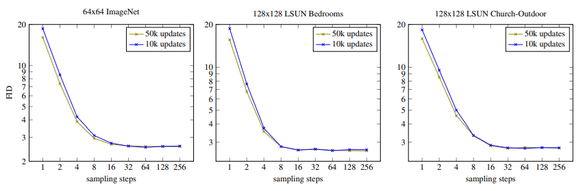
Fig. 418 50k updates vs 10k updates on ImageNet/LSUN datasets#