AffinityNet - CVPR 2018
Contents
AffinityNet - CVPR 2018#
Information
Title: Learning Pixel-level Semantic Affinity Image-level Labels for Weakly Supervised Semantic Segmentation, CVPR 2018
Reference
Review By: Taeyup Song
Edited by: Taeyup Song
Last updated on Jan. 5, 2022
Problem Statement#
Semantic segmentation model을 학습하기 위해서는 dense class label이 필요하지만, data를 수집하고 labeling 하는 것은 비용이 많이 든다.
Class Attention Map(CAM)을 활용하여 pseudo label 생성하고 이를 이용하여 semantic segmentation을 위한 network를 학습할 수 있지만, CAM이 sparse하고 blur한 정보이기 때문에 정확도가 떨어진다.
Contribution#
입력영상/CAM에서 semantic affinities(의미론적 유사도)를 계산하는 AffinityNet과 이를 기반으로 CAM에서 random walk를 이용하여 dense semantic label을 propagation하는 방법 제안.
Class label만 포함된 DB를 이용하여 생성한 pseudo label로 DeepLab model를 학습. VOC 12 test set 평가한 결과 weakly supervised learning 기반 방법 중 최초로 FCN보다 높은 mIoU를 달성함.
Background#
(1) Class Attention/Activation Map (CAM)
Classification을 위한 Network에서 특정 object에서 나타나는 특정한 pattern의 경우 score가 학습이 됨. 다양한 예제에서 공통적으로 나타나는 object들은 score가 낮게 학습이 됨.
discriminate 한 part에 집중하여 학습이 됨. (sparse하고 blurrly함. 외각영역에 집중되는 경향이 있음.)
instance-agnostic 함 ⇒ Pseudo Label로 바로 사용하기에는 한계가 있음
Proposed Method#
1. Key Idea#

Fig. 90 Illustration of our approach. (source: arXiv:1803.10464)#
Semantic affinity를 구하는 AffinityNet을 제안
AffinityNet으로 구한 Semantic affinity(동치관계)을 이용하여 CAM을 propagation하여 정확한 pseudo label을 생성 : Semantically identical한 area에는 propagation하고, 다른 class의 영역으로는 panalized 함.
생성된 pseudo label을 이용하여 semantic segmentation network(DeepLab)을 학습시킴.
2. CAM#
학습된 network가 주어졌을 때, groundtruth class \(c\)에 대한 CAM \(M_c\)은 다음과 같이 계산된다. computed by
\[M_c(x,y)=\mathbf{w}^{\top}_cf^{\text{cam}}(x,y)\]여기서 \(\mathbf{w}_c\) 는 class \(c\) classification weights이며, \(f^{\text{cam}}(x,y)\)는 \((x,y)\)위치의 GAP 이전 feature vector이다. \(M_c\)는 최대 activation이 1이 되도록 normalized 된다.
\[M_c(x,y) \rightarrow \frac{M_c(x,y)}{\max_{x,y}M_c(x,y)}\]어떤 class \(c'\)가 GT와 대응되지 않는 경우 무시하며, activation이 0이 되도록 만든다.
background activation map은 다음과 같이 계산된다.
\[M_{\text{bg}}=\{1-\max_{c\in C}M_c(x,y)\}^{\alpha}\]여기서 \(C\)는 set of object classes이며 \(\alpha\geq1\) 은 background confidence score를 조절하는 hyper-parameter이다.
CAM을 구하기 위한 Network는 ResNet38에 L4~L6를 dilated conv.로 변경한 backbone에 3x3 conv. layer와 GAP, FC를 추가한 network를 사용한다.
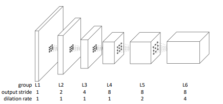
Fig. 91 Backbone network (source: arXiv:1803.10464)#
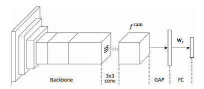
Fig. 92 Network for computing CAM (source: arXiv:1803.10464)#
3. AffinityNet#
(1) Architecture
ResNet38 backbone의 마지막 3개 layer를 dilated conv. layer로 변경하여 \(f^{\text{aff}}\)를 구함
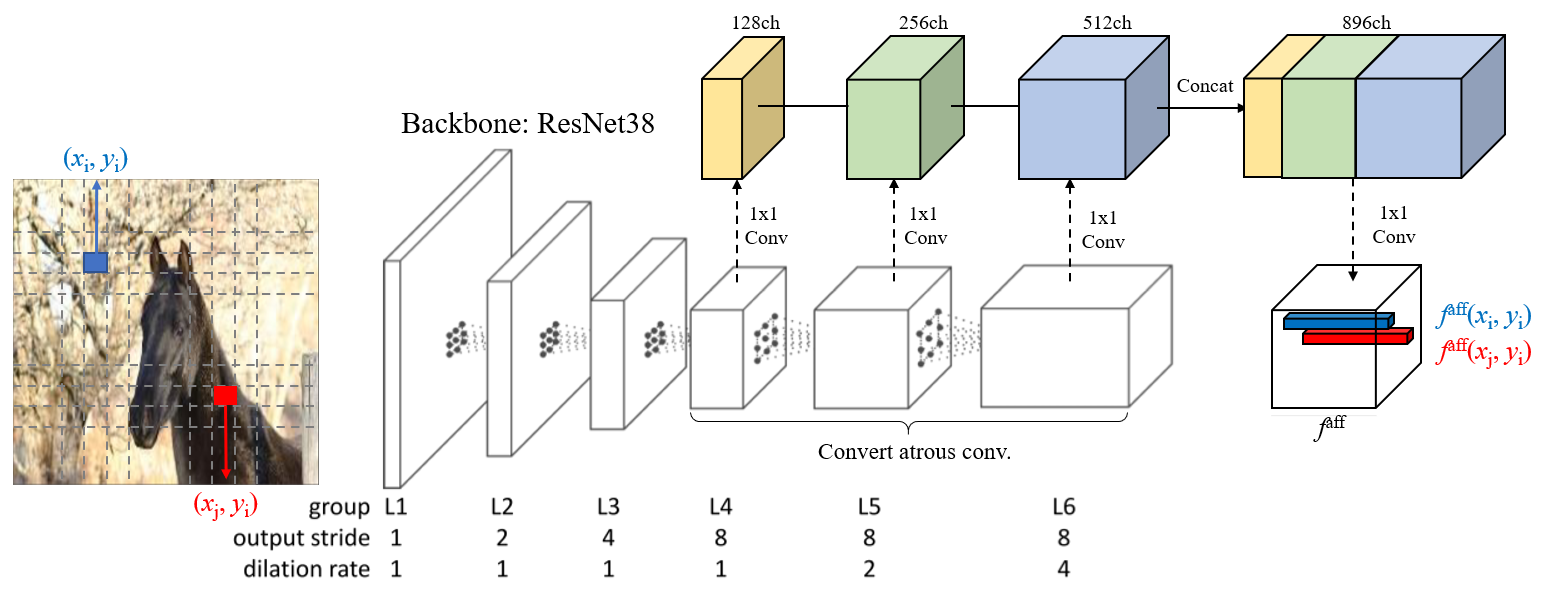
Fig. 93 AffinityNet architecture (modified from arXiv:1803.10464)#
feature \(i\)와 \(j\)에서의 semantic affinity \(W_{ij}\)는 두 위치의 affinity map \(f^{\text{aff}}\)의 pairwise \(L_1\)distance에 exponentiation 함수를 적용한 값을 사용
\[W_{ij}=\exp\{-||f^{\text{aff}}-f^{\text{aff}}(x_i,y_i)||_1\}\]두 feature가 같은 class label을 가지면 \(W_{ij}\)가 1이 되고, 아니면 0이 되도록 AffinityNet을 학습시킴.
(2) Learning AffinityNet
모든 pixel에 대해 pairing을 하면 computational cost가 너무 높기 때문에 전처리를 수행 후 뽑힌 pair에 대해 affinity label을 생성한다.
입력 영상에 대해 CAM을 추출
FG/BG를 각각 구분할 수 있도록 thresholding하고 dense CRF 후처리를 수행
여기서 threshold는 아주 보수적으로 설정함.
각 feature 위치에서 인접한 feature와의 pair를 구성하고, supervision으로 주어진 affinity label을 이용하여 학습
선정한 pair가 서로 같은 class를 가지는 positive affinity label과 서로 다른 class를 가지는 negative affinity label을 추출
FG/BG threshold의 중간 값을 가지는 feature(Figure 4에서 흰색 영역)는 affinity label 생성 시 사용하지 않음 (Don’t care)
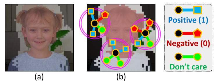
Fig. 94 Conceptual illustration of generating semantic affinity labels. (source: arXiv:1803.10464)#
Set of coordinate pairs \(\mathcal{P}\)는 다음과 같이 정의 가능하다.
\[\mathcal{P}=\{(i,j)|\text{d}\left((x_i,y_i),(x_j,y_j)\right)<\gamma, \forall i\neq j\}\]여기서 \(d\)는 Euclidean distance이고, \(\gamma\)는 pair가 가질 수 있는 최대 거리이다(거리검색 반경)
보통 object boundary에 negative pair가 편중되어 있고, 영상에서 객체보다 배경이 더 많기 때문에 class imbalance 문제가 발생함.
이를 해결하기 위해 우선 positive/negative subset으로 분리함.
\[\begin{split}\mathcal{P}^+=\{(i,j)|(i,j)\in\mathcal{P}, W_{i,j}^{*}=1\}, \\\mathcal{P}^-=\{(i,j)|(i,j)\in\mathcal{P}, W_{i,j}^{*}=0\},\end{split}\]positive subset \(\mathcal{P}^+\)를 객체/배경의 subset \(\mathcal{P}^+_{\text{fg}}\), \(\mathcal{P}^+_{\text{bg}}\) 로 한번 더 분리한다
AffinityNet의 Loss function은 다음과 같이 정의된다.
\[\mathcal{L}=\mathcal{L}^+_{\text{fg}}+\mathcal{L}^+_{\text{bg}}+2\mathcal{L}^-\]각 subset의 loss는 cross-entropy loss로 다음과 같이 정의된다.
\[\begin{split}\begin{aligned} \mathcal{L^+_{\text{fg}}}&=-\frac{1}{|\mathcal{P}^+_{\text{fg}}|} \sum_{(i,j)\in \mathcal{p}^+_{\text{fg}}}\log W_{ij} \\ \mathcal{L^+_{\text{bg}}}&=-\frac{1}{|\mathcal{P}^+_{\text{bg}}|} \sum_{(i,j)\in \mathcal{p}^+_{\text{bg}}}\log W_{ij} \\ \mathcal{L^-}&=-\frac{1}{|\mathcal{P}^-|} \sum_{(i,j)\in \mathcal{p}^-}\log (1-W_{ij}) \end{aligned}\end{split}\]Loss \(\mathcal{L}\)은 class-agnostic하다. 즉 학습된 AffinityNet은 class를 명시적으로 인식하지 못한 채 인접한 두 좌표가 클래스가 동일한지 여부(class consistency)만 판단한다. 따라서 general representation을 학습할 수 있게 된다.
4. Generating Pseudo Segmentation Labels#
Training image들의 CAM을 이용하여 학습된 AffinityNet이 주어지면, 이를 이용하여 local semantic affinities를 예측하고 transition probability matrix로 변환한다.
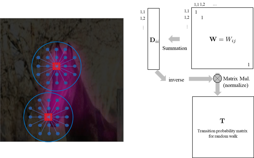
Fig. 95 Calculate transition probability matrix (modified from arXiv:1803.10464)#
Random walk에서 transition probability는 입력(CAM)에 대해 transition matrix \(T\)를 곱하는 형태로 구할 수 있다. → sementic affinity matrix는 각 coordinate pair로 구성되어 있으므로, CAM을 vectorize해서 multiply해야 dimension이 맞음.
이 과정을 \(t\)번 반복하여 semantic을 propagation한다.
5. Train Segmentation network#
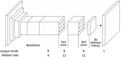
Fig. 96 Semantic segmentation network (source: arXiv:1803.10464)#
위 과정을 거처 생성한 semantic label은 입력 영상보다 작으므로, bilinear interpolation 및 dense CRF 후처리를 적용한 후 supervised learning 기반의 semantic segmentation network를 학습하는데 사용한다.
Experimental Result#
1. Implementation Details#
(1) Dataset: PASCAL VOC 2012 Benchmark
대부분의 weakly-supervised learning 기법에서 사용함
Super vision이 적고, Attention을 중점적으로 사용하기 때문에 COCO 같은 대용량 DB에서는 아직 성능이 낮게 나옴.
(2) Optimization
ImageNet pre-trained backbone
Adam optimizer를 이용하여 PASCAL VOC 2012로 finetune
(3) Data augmentation
모든 training image에 대해 horizontal flip, random cropping, color jittering 수행
AffinityNet이 scale invariant 하도록 학습하기 위해 input image를 random하게 scale조절
(4) Hyper parameter
Background attention map의 parameter \(\alpha\) 는 16을 기본값으로 4~24사이에서 가변
affinity search radius \(\gamma=5\)
Hadamard power of the original affinity matrix \(\beta=8\)
Number of iteration in random walk process \(t=256\)
2. Analysis of Synthesized Segmentation Labels#
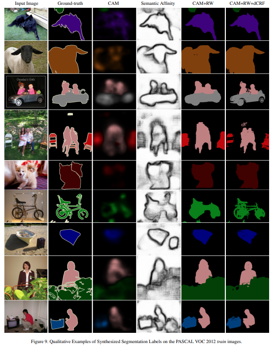
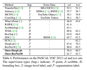
PASCAL VOC training set과 생성한 pseudo label을 mIoU로 비교한 결과 기존 방법대비 개선됨을 확인함.
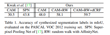
supervised learning으로 학슴한 FCN보다 높은 성능 나타냄 (fully supervision을 이용한 network보다 성능이 좋은 최초의 사례임.)
Semantic Affinity를 보면 AffinityNet이 의도한대로 object에 경계부분에 affinity score가 낮게 나옴을 알 수 있음.