MaX-DeepLab - CVPR 2021
Contents
MaX-DeepLab - CVPR 2021#
Information
Title: End-to-End Panoptic Segmentation with Mask Transformers, CVPR 2021
Reference
Review By: Jeunghyun Byun
Edited by: Taeyup Song
Last updated on Jun. 15, 2022
Contribution#
End-to-end panoptic segmentation 방법을 제안
기존의 방법들은 surrogate sub-task들 (e.g. box detection, anchor design rules, non-maximum suppression, 등등)을 포함한 pipeline을 사용함 (즉, hand-coded 된 prior에 의존)
MaX-DeepLab(Mask Xformer)은 Axial-DeepLab 모델을 확장한 것으로 mask transformer을 사용하고 bipartite matching으로부터 inspire된 loss을 사용함
Dual-path transformer 사용
COCO dataset에 대해서 새로운 test time augmentation을 적용하지 않고도 SOTA 성능을 확보함.
Background#
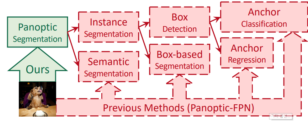
Fig. 83 Overview of Previous Method (Source: arXiv:2012.00759)#
기존의 panoptic segmentation method는 Fig. 83의 붉은색으로 표현된 내용과 같이 surrogate sub-task들에 의존하여 panoptic segmentation mask 결과를 구함.
즉 기존의 panoptic segmentation은 한번에 결과값을 구하는 것이 아니라 여러 task들로 구성되어 있는 다소 복잡한 pipeline 으로 구성되어 있다. (e.g. anchors, box assignment rules, non-maximum suppression, thing-stuff merging)
복잡한 pipeline으로 구성되어 각각의 surrogate task에서 “undesired artifact”가 발생할 수 있고 pipeline을 거치면서 더 큰 artifact / noise로 번질 수 있기 때문에 최근에는 pipeline을 간소화 하는 방향으로 여러 연구들이 소개되고 있다.
(1) Box Based Method in Panoptic Segmentation
Box based method는 Mask R-CNN과 같은 object detection 모델로 먼저 object bounding boxes들을 구하고 각 box안의 object에 해당되는 mask을 구한다. Instance segmentation과 Semantic segmentation가 서로 merge돼서 최종적인 panoptic segmentation을 구하게 된다.
대표적인 model: PanopticFPN, UPSNet, DETR(여전히 detection bounding box결과에 의존하는 한계를 가지고 있음), DetectoRS
(2) Box Free Method in Panoptic Segmentation
Box free method의 경우 먼저 semantic segment들을 구하고, 각각의 semantic segment에 속해 있는 pixel들을 group하여 instance segment들을 구한다.
Grouping 방법은 Instance Center Regression, Watershed transform, Hough-voting 그리고 Pixel affinity를 적용할 수 있다.
model: Axial-DeepLab (한계: challenges with highly deformable objects (which have a large variety of shapes) or nearby objects with close centers in the image)
Box based method. Box free method들 모두 일종의 “hand-coded prior”을 사용하므로 end-to-end pipeline이 아니다.
Proposed Method#
1. MaX-DeepLab formulation#
Panoptic Segmentation은 입력 영상 \(I \in \mathbb{R}^{H \times W \times 3}\)을 set of class-labeled mask로 분할하는 문제로 정의할 수 있다.
\[ \{\hat{y}\}_{i=1}^K=\{\left({m}_i,{c}_i\right)\}_{i=1}^K \]여기서 \(m_i\in \{0,1\}^{H \times W}\)는 서로 겹치지 않는 K개로 구성된 ground truth masks 이며, \(c_i\)는 mask \(m_i\)의 ground truth class label이다.
MaX-DeepLab은 \(N\)개의 output을 바로 도출하며, things와 staff class와 ∅(no class)로 구성되어 있어, ground truth 대비 큰 값으로 설정된다.
\[ \{\hat{y}\}_{i=1}^N={\left(\hat{m}_i,\hat{p}_i(c)\right)}_{i=1}^N \]여기서 \(\hat{m}_i\)은 predicted mask 이며, \(\hat{p}_i(c)\)는 mask \(\hat{m}_i\)가 \(c\) class에 속할 확률이다.
MaX-DeepLab은 end-to-end inference를 수행하기 때문에 별도의 post-processing 없이 두 번의 간단한 softmax 연산으로 panoptic segmentation 결과를 얻을 수 있다.
각 mask에 대해 class label을 predict
\[ \hat{c}_i=\arg\max_c \hat{p}_i(c) \]모든 pixel에 대해 mask-ID를 predict
2. Model Architecture#
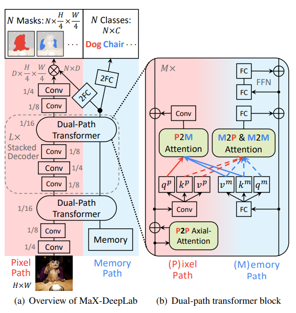
Fig. 84 An overview of the dual-path transformer architecture (Source: Source: arXiv:2012.00759)#
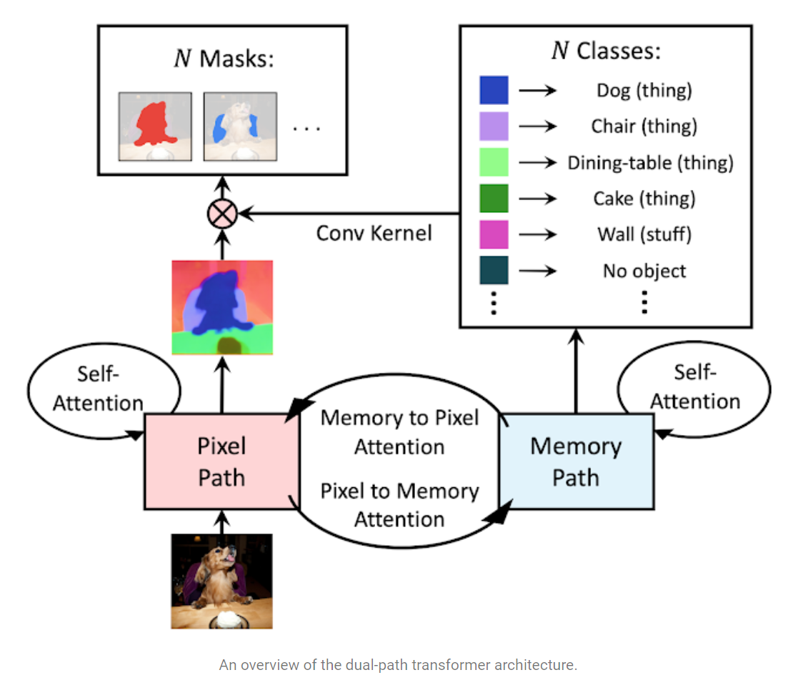
Fig. 85 Overview of MaX-DeepLab (Source: https://ai.googleblog.com/2021/04/max-deeplab-dual-path-transformers-for.html)#
MaX-DeepLab은 dual-path transformer, stacked decoder, output heads (for mask and classes prediction)으로 구성된다.
(1) Dual-path Transformer
Axial-attention blocks을 적용함.
mask prediction을 위한 2D pixel-based CNN \((H \times W \times d_{in})\)으로 구성된 pixel path와 class prediction 및 mask생성을 위한 1D global memory \((N \times d_{in})\) path로 구성되어 있다.
각 path에 따라 다음과 같은 attention을 활용한다.
memory-to-pixel (M2P) attention (일반적인 attention)
memory-to-memory (M2M) self-attention
pixel-to-memory (P2M) feedback attention
pixel-to-pixel (P2P) self-attention (axial attention blocks)
입력 영상에 대해 conv. layer를 통해 얻은 2D input feature \(x^p \in \mathbb{R}^{\hat{H} \times \hat{W} \times d_{in}}\)와 1D global memory feature \(x^m\in\mathbb{R}^{M \times d_{in}}\)이 주어질 때, pixel position \(a\)에서의 feedback attention’s output **(Pixel-to-memory)**은 다음과 같이 나타낼 수 있다.
Memory-to-pixel (M2P) and memory-to-memory (M2M) attention 출력은 다음과 같다.
\[\begin{split} \begin{aligned} q_b^m&=\sum_{n=1}^{\hat{H}\hat{W}+N}\text{softmax}_n(q_a^p\cdot k_n^m)v_n^m,\\ &k^{\text{pm}}=\left[\begin{matrix}k ^p \\k^m \end{matrix}\right], v^{\text{pm}}=\left[\begin{matrix}v^p \\v^m \end{matrix}\right] \end{aligned} \end{split}\]
(2) Stacked Decoder
light-weight decoder가 아닌 hourglass 스타일의 stacked decoder를 적용함.
\(L\)개의 decoder를 stack한 구조를 적용하며 (4, 8 and 16 output strides) feature는 bilinear interpolation 후 단순 합 연산으로 fuse한다.
(3) Output heads
Memory Path output을 이용하여 다음을 추정한다.
2개의 fully connected layers (2FC)를 거쳐 \(N\)개의 mask classes \(\hat{p}(c)\in\mathbb{R}^{N\times|\mathbb{C}|}\)를 추정한다.
또다른 2FC를 이용하여 mask features \(f\in\mathbb{R}^{N\times D}\)를 추정한다.
Pixel Path의 decoder output(stride 4)을 이용하여 다음을 생성한다.
2번의 convolutions을 거쳐 normalized feature \(g\in \mathbb{R}^{D \times \frac{H}{4} \times \frac{W}{4}}\)를 생성
최종 mask \(\hat{m}\)은 다음과 같이 mask feature \(f\)와 decoder feature \(g\)의 간단한 곱으로 구한다.
\[ \hat{m}=\text{softmax}_N(f\cdot g)\in \mathbb{R}^{N\times\frac{H}{4}\times\frac{W}{4}} \]Mask prediction 과정은 CondInst and SOLOv2 모델에 영감을 받았지만, 두 방법이 hand-designed object centers와 things와 stuff mask의 merge가 필요한 반면 제안된 방법은 end-to-end 방식으로 mask prediction을 추정할 수 있다.
3. PQ-style loss#
Model을 학습하기 위해 panoptic quality (PQ)의 정의를 활용한 PQ-style loss를 이용한다. PQ는 다음과 같이 recognition quality(RQ)와 segmentation quality(SQ)로 정의된다.
(1) Mask similarity metric
Class-labeled ground truth mask \(y_i=(m_i,c_i)\)와 prediction \(\hat{y}_j=(\hat{m}_j, \hat{p}(c))\)과의 mask similarity metric은 다음과 같이 정의된다.
\[ \text{sim}\left(y_i,\hat{y}_j\right)=\underbrace{ \hat{p}_j(c_j)}_{\approx\text{RQ}} \times \underbrace{ \text{Dice}(m_i,\hat{m}_i)}_{\approx\text{SQ}} \]여기서 \(\hat{p}_j (c_i) \in [0,1]\)는 올바른 class로 예측한 경우의 probability이며, \(\text{Dice}(m_i,\hat{m}_j)\)의 경우 GT와 prediction mask간의 Dice coefficient이다.
mask similarity는 class prediction이 틀리거나, GT와 prediction mask가 overlap이 안되는 경우 0의 최소값을 가지며, class prediction이 정확하고, mask가 정확히 일치하면 1의 최대값을 가진다.
(2) Mask Matching
predicted mask와 각 GT mask를 matching하기 위해 prediction set \(\{\hat{y}_i\}_{i=1}^N\)과 GT set \(\{y_i\}_{i=1}^K\)간의 one-to-one bipartite matching problem을 정의하고 해를 구한다. GT와의 total similarity가 최대가 되는 prediction을 assign한다.
\[ \hat{\sigma}=\arg\max_{\sigma\in \mathfrak{S}n}\sum_{i=1}^{K}\text{sim}(y_i,\hat{y}_{\sigma(i)}) \]\(K\) matches predictions = positive masks
\((N-K)\) masks left = negative masks (i.e. no object)
기존 연구(DETR)과 같이 Hungarian algorithm을 적용하여 최적의 match를 찾는다.
DETR의 경우 NMS를 사용하지 않고 중복되는 boxes를 제거하기 위해 단 1개의 positive matching만을 허용함.
MaX-Deeplab 모델의 경우 중복되거나 overlaped 된 mask는 설계상 존재할 수 없음.
하지만 하나의 GT mask에 여러개의 predicted mask가 할당되는 것은 최적화 관점에서 문제가 될 수 있음. (하나의 GT mask에 2개의 predicted mask가 예측되는 경우)
(3) PQ-style loss
Match되는 masks(positive masks)에 대해 다음과 같이 PQ-style objective function을 최대화 하는 parameter \(\theta\)를 찾는 최적화 문제를 정의한다.
\[ \max_{\theta}\mathcal{O}_{\text{PQ}}^{\text{pos}}= \sum_{i=1}^{K} \underbrace{ \hat{p}_{\hat{\sigma}(i)}(c_i) }_{\approx\text{RQ}} \times \underbrace{ \text{Dice}(m_i,\hat{m}{\hat{\sigma}(i)}) }_{\approx\text{SQ}} \]Objective function \(\mathcal{O}^{\text{pos}}\)에 product rule of gradient를 적용하고, 최적화에 유리하도록 predicted probability에 log를 취해 cross-entropy 형태로 치환하여 matched mask에 대한 loss로 적용한다.
\[\begin{split} \begin{aligned} \mathcal{L}_{\text{PQ}}^{\text{pos}}&= \sum_{i=1}^{K} \underbrace{ \hat{p}_{\hat{\sigma}(i)}(c_i) }_{\text{weight}} \cdot \underbrace{ \left[-\text{Dice}(m_i,\hat{m}_{\hat{\sigma}(i)})\right] }_{\text{Dice loss}} \\ &+\sum_{i=1}^{K} \underbrace{ \text{Dice}(m_i,\hat{m}_{\hat{\sigma}(i)}) }_{\text{weight}} \cdot \underbrace{ \left[-\log \hat{p}_{\hat{\sigma}(i)}(c_i)\right] }_{\text{Cross-entropy loss}} \end{aligned} \end{split}\]Dice loss는 class correctness를 최적화 하고, cross-entropy는 mask correctness를 최적화 한다. 만약 잘못된 mask와 match된 경우 class weight를 감소시게 된다.
Unmatched mask의 경우 cross-entropy loss를 적용한다.
\[ \mathcal{L}_{\text{PQ}}^{\text{neg}}=\sum_{i=K+1}^{N}\left[-\log \hat{p}_{\hat{\sigma}(i)}(∅)\right] \]최종적으로 다음과 같은 loss를 학습에 적용한다.
\[ \mathcal{L}_{\text{PQ}}=\alpha\mathcal{L}_{\text{PQ}}^{\text{pos}}+(1-\alpha)\mathcal{L}_{\text{PQ}}^{\text{neg}} \]
4. Auxiliary Losses#
학습 과정에서 PQ-style loss와 더불어 auxiliary losses를 적용했을 때 이득이 있음을 확인함.
(1) Instance discrimination
Decoder feature \(g\in \mathbb{R}^{D \times \frac{H}{4} \times \frac{W}{4}}\)가 instance로 clustering 되도록 함.
첫번째로 decoder feature와 동일한 resolution으로 downsample된 GT mask \(m_i \in \{0,1\}^{\frac{H}{4} \times \frac{W}{4}}\)가 주어지면, mask \(m_i\)내부의 \(K\)개의 annotated maak에 대해 average feature embedding \(t_{i,:} \in \mathbb{R}^D\)를 구함
\[ t_{i,:}=\frac{\sum_{h,w}m_{i,h,w} \cdot g_{:,h,w}}{||\sum_{h,w}m_{i,h,w} \cdot g_{:,h,w}||}, \ i=1,2,...,K \]각 pixel의 feature \(g_{:,h,w}\)에 대해 instance discrimination task를 수행한다.
\[ \mathcal{L}_{h,w}^{\text{InstDis}}=-\log \frac{\sum_{i=1}^K m_{i,h,w}\exp(t_{i,:}\cdot g_{:,h,w}/\tau)}{\sum_{i=1}^K \exp(t_{i,:}\cdot g_{:,h,w}/\tau)} \]여기서 \(\tau\)는 temperature 값이며, \(m_{i,h,w}\)는 0이 아닌 값으로 i번째 instance를 포함하는 mask \(m_i\)에 속한 값이다.
이 loss값은 모든 instance pixel에 적용되어 동일한 instance의 feature가 유사한 값을 가지고, 서로 다른 instance feature가 구분되는 값을 같도록 학습되게 한다.
(2) Mask-ID Cross-Entropy
Inference 과정에서 mask ID map이 주어지면 이를 이용하여 classification task에 적용되는 cross-entropy loss를 추가로 계산하여 학습에 사용한다.
(3) Semantic Segmentation
각 pixel의 semantic feature를 추출하기 위해 backbone의 output에 Panoptic-DeepLab model의 semantic head를 연결함.
semantic head를 첫번째 decoder(stride 4)에 연결했을 때 최종 mask feature를 분리하는데 도움이 됨을 확인함.
Experimentation Result#
1. Tech. details#
Computing resources: 32 TPU cores for 100k iterations (54 epochs)
RAdam, Lookahead optimizer with “poly” schedule
Output: \(N=128\), \(D=128\) channels
Data: COCO val set and test-dev set
Models:
Max-DeepLab-L (Wide-ResNet-41, L=2 stacking)
Max-DeepLab-S (ResNet-50 with axial attention blocks, no stacking L=0)
2. Result#
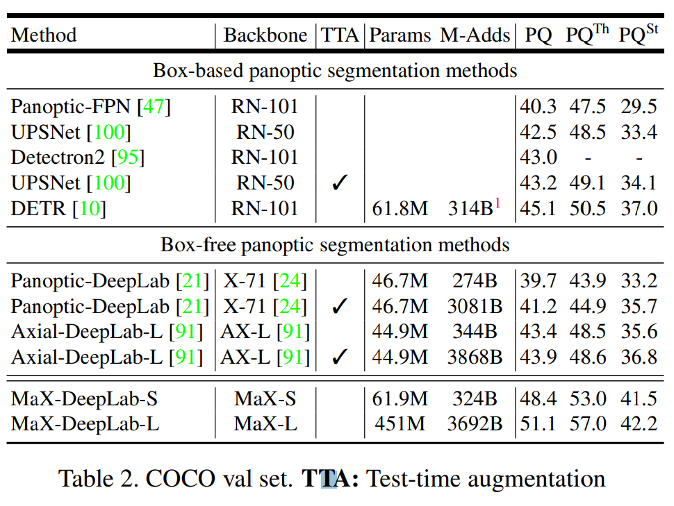
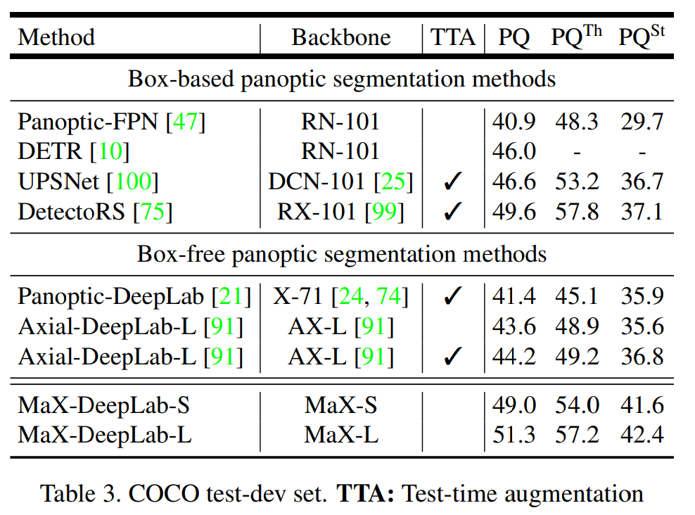
COCO val. set과 test-dev set에서 single-scale model인 MaX-DeepLab-S가 기존 box-based method 및 box-free method 대비 높은 PQ를 나타냄.
Test-time augmentation을 사용하지 않고도 SOTA 성능을 확보함.