BCNet - CVPR 2021
Contents
BCNet - CVPR 2021#
Information
Title: Deep Occlusion-Aware Instance Segmentation with Overlapping BiLayers, CVPR 2021
Reference
Review By: Hwigeon Oh
Last updated on Aug. 13, 2022
Introduction#
Mask R-CNN 형태의 instance segmentation은 box prediction을 수행 후 instance masks를 추출하는 과정을 거친다.
하지만 각 instance에 대해 개별적으로 추출된 ROI feature에서 regression되는 구조는 overlap된 objects, 특히 같은 class에 속한 objects가 overlap되었을 때, 많은 segmentation error를 확인할 수 있다.
이러한 문제를 해결하기 위해 NMS와 추가적인 후처리(post processing)를 추가한 모델이 제안되었으나, 경계가 과하게 smoothing되거나 instance간의 약간의 gap이 발생하는 문제 가 있었다.
Fig. 67.(d)와 같ASN과 같이 amodal/occlusion mask prediction을 위한 network의 경우 겹침이 발생한 object(occludee)에만 집중하여 성능의 한계가 존재한다.
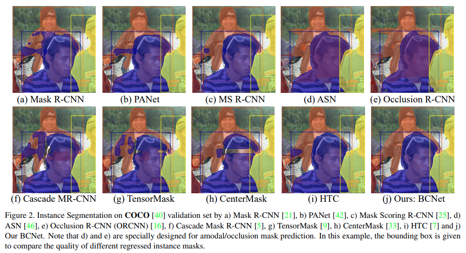
Fig. 67 Instance Segmentation on COCO (source: arXiv:2103.12340)#
본 논문에서는 occluder / occludee을 각각 처리하는 layer로 구성하고, 두 layer의 interaction 활용하는 Bilayer Occluder-Occludee structure를 제안한다.
Proposed Method#
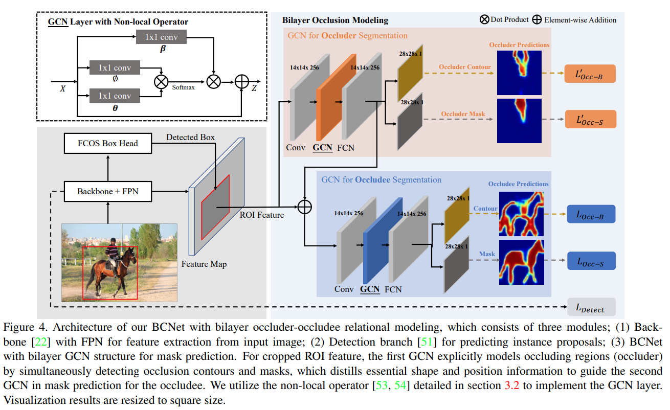
Fig. 68 Architecture of BCNet with bilayer occluder-occludee relational modeling (source: arXiv:2103.12340)#
영상 내에서 Heavy occlusion된 두 instance는 동일한 bounding box를 가지게 되며, contour를 확인하기 어렵다.
이런 한계를 극복하기 위해 제안 본 논문에서는 기존에 제안된 two-stage instance segmentation 방법을 확장한 BCNet architecture를 제안한다. BCNet은 다음과 같이 구성된다.
(1) ROI feature extraction을 위한 backbone과 FPN
(2) 각 Instance proposal의 bounding box를 예측하기 위한 object detection head (FCOS 적용)
(3) Bilayer GCN(Graph Convolutional Network)로 구성된 occlusion-aware mask head
→ Occluder/occludee에 대해 2개의 layer로 정의되며, mask와 contour prediction을 수행하도록 구성.
1. Bilayer Occluder-Occludee Modeling#
(1) Bilayer GCN Structure for Instance Segmentation
Overlap 비율이 높은 object의 경우 겹쳐진 (occluded) object에 의해 분할되거나 겹침이 발생하여 작게 표시될 수 있으므로, occlusion에 잘 대응하기 위해 mask head의 기본 block으로 long-range relationship을 반영할 수 있는 GCN을 적용한다.
Edges \(\mathcal{E}\)와 nodes \(\mathcal{V}\)로 구성된 인접 graph (adjacency graph) \(\mathcal{G}=\langle\mathcal{V,\mathcal{E}}\rangle\) 가 주어졌을 때, Graph Convolution operation은 다음과 같이 표현할 수 있다.
\[ Z=\sigma(AXW_g)+X \]여기서 \(X\in \mathbb{R}^{N\times K}\) 은 input feature이며, \(N=H×W\) 은 ROI region 주변의 pixel grids의 수를 나타낸다. \(A\in \mathbb{R}^{N\times N}\) 는 adjacency matrix, \(W_g\in \mathbb{R}^{K\times K′}\) 는 학습 가능한 weight matrix를 나타낸다.
Adjacency matrix \(A\)를 구성하기 위해 모든 dot product similarity를 이용하여 graph node 사이의 pairwise similarity를 정의한다.
\[\begin{split} A_{ij}=\text{softmax}(F(\mathbf{x}_i,\mathbf{x}_j)) \\ F(\mathbf{x}_i,\mathbf{x}_j)=θ(\mathbf{x}_i)^T \phi(\mathbf{x}_j) \end{split}\]여기서 \(\theta\) 와 \(\phi\) 는 \(1\times 1\) convolution으로 구현되는 transformation function으로 feature간의 큰 similarity가 커지면 edge의 confidence가 커지도록 학습된다.
Adjacency matrix의 경우 Attention과 동일한 형태임을 code를 통해 확인할 수 있다.
# https://github.com/lkeab/BCNet/blob/main/detectron2/modeling/roi_heads/mask_head.py#L411

# x: B,C,H,W
# x_query: B,C,HW
x_query_bound = self.query_transform_bound(x).view(B, C, -1)

# x_query: B,HW,C
x_query_bound = torch.transpose(x_query_bound, 1, 2)

# x_key: B,C,HW
x_key_bound = self.key_transform_bound(x).view(B, C, -1)

# x_value: B,C,HW
x_value_bound = self.value_transform_bound(x).view(B, C, -1)

# x_value: B,HW,C
x_value_bound = torch.transpose(x_value_bound, 1, 2)

# W = Q^T K: B,HW,HW
x_w_bound = torch.matmul(x_query_bound, x_key_bound) * self.scale
x_w_bound = F.softmax(x_w_bound, dim=-1)

# x_relation = WV: B,HW,C
x_relation_bound = torch.matmul(x_w_bound, x_value_bound)

# x_relation = B,C,HW
x_relation_bound = torch.transpose(x_relation_bound, 1, 2)

# x_relation = B,C,H,W
x_relation_bound = x_relation_bound.view(B,C,H,W)
x_relation_bound = self.output_transform_bound(x_relation_bound)
x_relation_bound = self.blocker_bound(x_relation_bound)

x = x + x_relation_bound
저자가 제안한 bilayer GCN 구조의 output feature는 다음과 같이 구성된다.
\[\begin{split} Z^1=\sigma(A^1X_fW_g^1)+X_f \\ X_f=Z^0W_f^0+X_{roi} \\ Z^0=\sigma(A^0 X_{roi}W_g^0)+X_{roi} \end{split}\]여기서 \(\mathcal{G}^i\) 는 \(i\)번째 graph, \(X_{roi}\)는 입력되는 ROI feature, \(\mathbf{W}_f\) 는 mask head에 적용되는 FCN layer의 weights이다.
Occluder feature (\(Z^0\))를 추출한 후 이를 이용하여 Occludee feature(\(Z^1\))를 만들 때 사용한다.
각 pixel의 binary label(Foreground/background)을 추정하는 기존 single layer 구조의 class-agnostic mask head와 비교하여 bilayer GCN의 경우 추가적으로 겹치는 영역에 대한 semantic graph space를 제공한다.
(2) Occluder-occludee Modeling
Occluder의 boundary detection은 다음과 같은 loss를 이용하여 학습된다.
\[ \mathcal{L}'_{\text{Occ-B}}=\mathcal{L}_{\text{BCE}}(W_B\mathcal{F}_{occ}(\mathbf{X}_{roi}),\mathcal{GT}_B) \]여기서 \(\mathcal{L}_{\text{BCE}}\)는 binary cross-entropy loss, \(\mathcal{F}_{occ}\)는 occlusion modeling module의 nonlinear transformation function, \(W_B\)는 boundary predictor weight, \(\mathbf{X}_{roi}\)는 ROI Alignd을 통해 cropped된 target 영역의 FPN feature map을 나타내며, \(\mathcal{GT}_B\)는 mask annotation을 통해 미리 계산된 occluder의 boundary이다.
Occluder의 mask prediction은 shared feature \(\mathcal{F}_{occ}(\mathbf{X}_{roi})\) 를 이용하며, boundary prediction과 함게 최적화된다. segmentation loss는 다음과 같이 modeling된다.
\[ \mathcal{L}'_{\text{Occ-S}}=\mathcal{L}_{\text{BCE}}(W_S\mathcal{F}_{occ}(\mathbf{X}_{roi}),\mathcal{GT}_S) \]여기서 \(W_S\) 학습 대상인 segmentation mask predictor의 weight이며, \(\mathcal{GT}_S\)는occluder의 mask annotation이다.
2. End-to-end Patameter Learning#
제안된 instance segmentation framework은 multi-task loss function을 이용하여 end-to-end로 학습된다.
\[\begin{split} \mathcal{L}=\lambda_1 \mathcal{L}_{\text{Detect}}+\mathcal{L}_{\text{Occluder}}+\mathcal{L}_{\text{Occludee}}, \\ {L}_{\text{Occluder}}=\lambda_2 \mathcal{L}'_{\text{Occ-B}}+\lambda_3 \mathcal{L}'_{\text{Occ-S}},\\ {L}_{\text{Occludee}}=\lambda_4 \mathcal{L}_{\text{Occ-B}}+\lambda_5 \mathcal{L}_{\text{Occ-S}}, \end{split}\]여기서 \(\lambda\) 는 hyper-parameter weight로 validataion set을 이용하여 튜닝한 값을 적용한다.
Backbone ~ RoI Head는 FCOS를 사용했다.
\[ \mathcal{L}_{\text{Detect}}=\mathcal{L}_{\text{Regression}}+\mathcal{L}_{\text{Centerness}}+\mathcal{L}_{\text{Class}} \]
[Note]
Occluder region은 offline으로 미리 산출 후 학습에 적용한다.
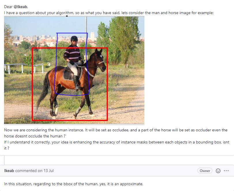
Target object를 occludee로 설정하고, target object의 bounding box안에 존재하는 다른 object pixel을 전부 union 하는 것으로 occluder region를 구한다.
# https://github.com/lkeab/BCNet/blob/main/detectron2/data/datasets/process_dataset.py#L254:L296

for index1, a_box in enumerate(box_list):
	union_mask_whole = np.zeros((int(img_dict["height"]), int(img_dict["width"])), dtype=int)
	for index2, b_box in enumerate(box_list):
		if index1 != index2:
			iou = bb_intersection_over_union(a_box, b_box)
			if iou > 0.05:
				union_mask = np.multiply(box_mask_list[index1], bitmask_list[index2])
				union_mask_whole += union_mask

	print("===========================================")
	print('bit mask area:', bitmask_list[index1].sum())
	union_mask_whole[union_mask_whole > 1.0] = 1.0
	print('cropped union mask area:', union_mask_whole.sum())
	intersect_mask = union_mask_whole * bitmask_list[index1]
	print('intersect mask area:', intersect_mask.sum())
	print('intersect rate:', intersect_mask.sum()/float(bitmask_list[index1].sum()))
	print("===========================================")

	if intersect_mask.sum() >= 1.0:
		intersect_num += 1

	if float(bitmask_list[index1].sum()) > 1.0:
		intersect_rate += intersect_mask.sum()/float(bitmask_list[index1].sum())

	union_mask_non_zero_num = np.count_nonzero(union_mask_whole.astype(int))
	record["annotations"][index1]['bg_object_segmentation'] = []
	if union_mask_non_zero_num > 20:
		sum_co_box += 1
		contours = measure.find_contours(union_mask_whole.astype(int), 0)
		for contour in contours:
			if contour.shape[0] > 500:
				contour = np.flip(contour, axis=1)[::10,:]
			elif contour.shape[0] > 200:
				contour = np.flip(contour, axis=1)[::5,:]
			elif contour.shape[0] > 100:
				contour = np.flip(contour, axis=1)[::3,:]
			elif contour.shape[0] > 50:
				contour = np.flip(contour, axis=1)[::2,:]
			else:
				contour = np.flip(contour, axis=1)

			segmentation = contour.ravel().tolist()
			record["annotations"][index1]['bg_object_segmentation'].append(segmentation)
따라서, 실제로는 occlusion이 일어나지 않아도 occluder가 될 수 있다. (참고: link)
이후 occluder region은 ground truth로 이용된다.
Boundary ground truth는 online으로 구한다.
https://github.com/lkeab/BCNet/blob/main/detectron2/modeling/roi_heads/mask_head.py#L83:L89
https://github.com/lkeab/BCNet/blob/main/detectron2/layers/boundary.py#L38:L59
https://github.com/lkeab/BCNet/blob/main/detectron2/layers/boundary.py#L12:L26
Experiments#
1. Implementation Details#
Train dataset
COCO 2017train (115k images)
첫번째 GCN layer를 학습하기 위해 COCO set 중에서 occlusion cases가 50%이상 구성되도록 ROI proposal을 filtering 함.
ResNet-50-FPN backbone을 적용하고, 입력 영상의 경우 aspect ratio가 변하지 않도록 600 pixel(짧은쪽)/ 900pixel(긴쪽)이 넘지 않도록 resize 함.
2. Experimental Result#
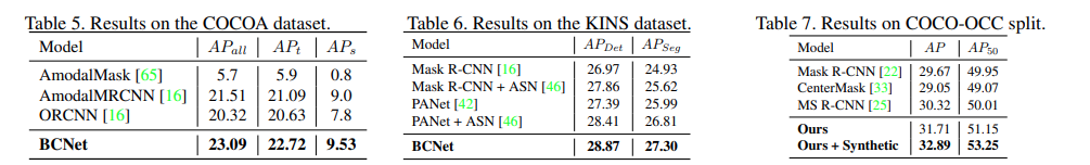
COCO test-dev에서 당시 SOTA method와 비교한 결과 PANet 및 Mask Scoring R-CNN보다 개선된 성능을 나타냄. BCNet은 3단계의 cascade refinement와 더 많은 parameter를 사용한 HTC와 유사한 성능을 나타내어 기존 방법 대비 효율적으로 높은 성능을 나타냄을 확인 할 수 있음.
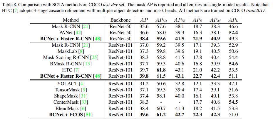
Occlusion 대응을 비교하기 위해 저자가 제안한 COCO-OCC split에서 다른 Two-stage instance segmentation model 대비 높은 성능을 나타냄