2.4. Recovery of affine and metric properties from images

2.4. Recovery of affine and metric properties from images#

The Method to recover similarity properties from projective distored images#

평면에 projection되어 있는 이미지에서 사영 왜곡을 제거하면 각도, 길이 비율과 같은 similarity 속성을 원래 평면에서 측정할 수 있으며, 4개의 대응점을 지정하여 dof가 8인 projective transformation H를 계산해 사영 왜곡을 완전히 제거할 수 있습니다.

그러나 similarity transformation은 projective tranformation에 비해 dof가 4개 더 적습니다. 따라서 4 dof만 지정하여도 similarity 속성을 측정할 수 있습니다.

사영 왜곡된 이미지에서 similarity 속성을 복원하기 위한 4개의 dof는 line at infinity $l_{\infty}$ (dof 2)와 $l_{\infty}$ 에 있는 두 개의 원형점( $c i r c u l a r p o i n t s$ , dof 2)이라는 물리적 실체로 주어지며, 이러한 연관성을 이용하는 것이 행렬 분해에서 나타나는 행렬을 지정하는 방식보다 문제를 더 직관적으로 해결할 수 있습니다.

이미지에서 $l_{\infty}$ 가 결정되면 사영 왜곡을 제거할 수 있고, $c i r c u l a r p o i n t s$ 가 결정되면 아핀 왜곡을 제거할 수 있습니다. 그러면 남은 왜곡은 similarity 뿐이므로, 이미지에서 similarity 속성을 측정할 수 있습니다.

2.4.1 The line at infinity#

사영 변환에 의해 왜곡된 이미지에서 무한선(the line at infinity) $l_{\infty}$ 을 식별하면 아핀 속성을 복원할 수 있습니다. 그 이유는 line at infinity $l_{\infty}$ 이 projective transformation H에 invariant하기 때문입니다.

figure2.7_1 figure2.7_1-2

2.4.2 Recovery of affine properties from images#

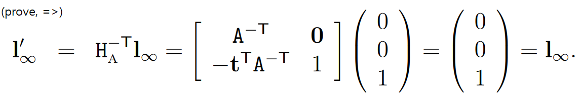
사영 변환에 의해 왜곡된 이미지에서 line at infinity $l_{\infty}$ 을 식별하여 line at infinity의 표준 위치인 $(0, 0, 1)^{T}$ 로 보내는 변환을 적용하면, Result 2.17.에 의해 이미지에 적용된 변환은 아핀 변환임을 보일 수 있습니다.

즉 이미지의 아핀 속성을 복원한 것입니다. 다음 그림에서 이 핵심 아이디어에 대해 잘 설명하고 있습니다. 그렇다면 사영 변환에 의해 왜곡된 이미지에서의 line at infinity $l_{\infty}$ 을 식별하는 방법은 무엇이 있을까요?

이 책에서는 2가지 방법을 소개합니다.

평행선의 교점을 이용한 방법
길이 비율을 이용한 방법

위 두 가지 중 저희는 1번 방법에 대한 실습을 함께 제공합니다.

Affine rectification#

아래 이미지는 3가지의 평면과 그 사이에서의 일어날 수 있는 2가지 변환으로 아핀 속성이 보정되는 과정을 보입니다. 3가지 평면은 왼쪽부터 순차적으로 아래와 같은 평면을 나타냅니다.

실제 세계에서 왜곡 없이 평면으로 사영된 평면 $π_{1}$ ,
projective transformation에 대해 변환되어 사영된 평면 $π_{2}$ ,
$π_{2}$ 에서 아핀 속성을 복원한 $π_{3}$

또한, $H_{P}$ 는 projective transformation, $H_{A}$ 는 Affine transformation 입니다.

figure2.7_3

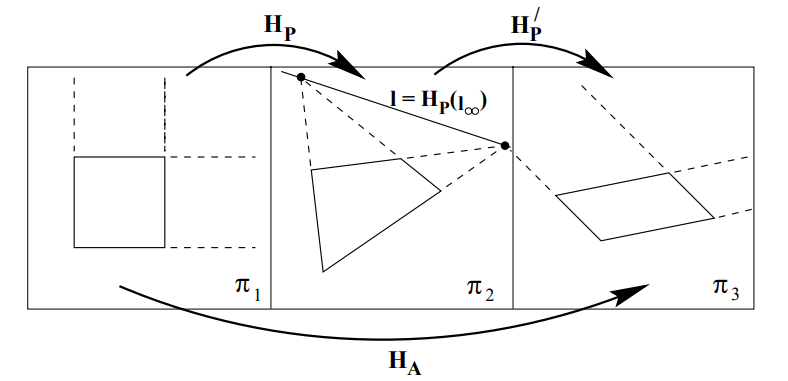
위 그림에서 알 수 있는 것은 2가지입니다.

projective transform에 의해 왜곡된 이미지에서 line at infinity $l_{\infty}$ 을 식별하여 affine 속성을 복원해 평행인 것을 평행으로 만들 수 있다는 것
위와 같이 복원된 평면은 원본과 affine transforation의 관계를 가진다는 것

The Method using the intersection of parallel lines#

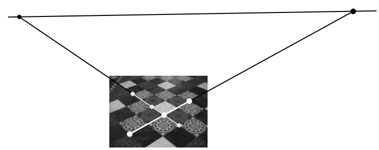
실세상 평면의 line at infinity는 원근 이미지에서 평면의 vanishing line이 됩니다. 다음 그림에서 나와있듯이, vanishing line $l$ 은 이미지에서 평행선의 교점에서 계산할 수 있습니다.

figure2.7_4

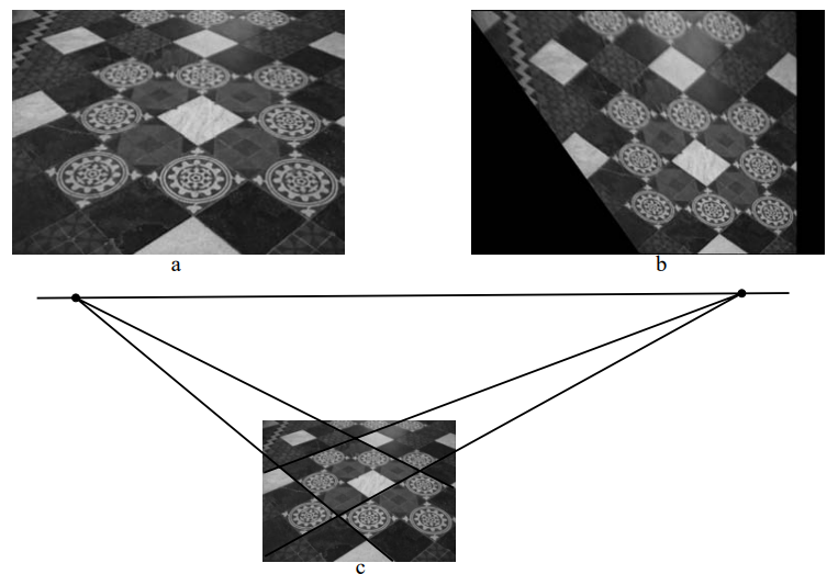
vanishing line을 식별하는 방법을 요약해보겠습니다.

실제 세계에서는 평행한 두 직선을 2 pair 찾습니다.
외적을 이용해서 각 쌍에 존재하는 두 직선의 접점을 계산합니다.
위 과정을 통해 구한 2개의 접접의 외적을 이용해 선의 좌표 계산합니다.

아래 실습 코드가 있습니다.

import numpy as np
import cv2

import matplotlib.pyplot as plt

img = cv2.imread('./figures/chessboard.jpg', cv2.IMREAD_COLOR)

st = [np.array([1381,  969]), np.array([1719,  392]), np.array([337, 711]), np.array([1382,  968])]
ed = [np.array([338, 711]), np.array([786, 195]), np.array([786, 194]), np.array([1719,  392])]
# Homogeneous vectorize
st = np.append(st, np.ones((4,1), dtype=np.int32), axis=1)
ed = np.append(ed, np.ones((4,1), dtype=np.int32), axis=1)

# Compute vanishing point Vx
Vx = np.cross(np.cross(st[0], ed[0]),np.cross(st[1], ed[1]))
Vx = Vx/Vx[2]

# Compute vanishing point Vy
Vy = np.cross(np.cross(st[2], ed[2]),np.cross(st[3], ed[3]))
Vy = Vy/Vy[2]

# Compute vanishing line Vl
Vl = np.cross(Vx,Vy)
Vl = Vl/Vl[2]
print('Vanishing line : ', Vl)

# compute affine rectification matrix
H_A = np.eye(3)
H_A[2] = Vl

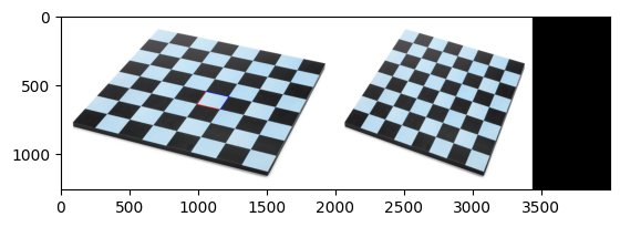
# recover the affine properties
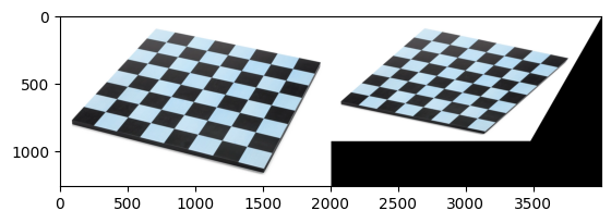
recovered_img = cv2.warpPerspective(img, H_A, (0,0))

concat = np.concatenate([img, recovered_img], axis=1)
plt.imshow(concat)

Vanishing line :  [6.61317266e-07 2.85906628e-04 1.00000000e+00]

<matplotlib.image.AxesImage at 0x168e874d0>

../../_images/92bfb51d20554986b6691046a659ddd487f1a8119b5a2eef2ed112638126acde.png

Computing a vanishing point from a length ratio#

또는 길이 비율이 알려진 두 개의 간격이 주어지면 소실점을 결정할 수 있습니다. 일반적인 경우는 이미지의 한 직선에서 세 점이 식별된 경우입니다. $a, b, c$ 가 실세계에서 대응하는 같은 선상의 점이고, 길이 비율 $d (a, b) : d (b, c) = a : b$ 가 알려져 있다고 가정합니다. 교차 비율을 사용하면 소실점을 찾아낼 수 있습니다.

figure2.7_5

이미지에서 거리 비율 $d (a^{'}, b^{'}) : d (b^{'}, c^{'}) = a^{'} : b^{'}$ 을 측정합니다.
점 $a, b, c$ 를 직선 $< a, b, c >$ 상의 좌표계에서 좌표 $0, a, a + b$ 로 표기합니다. 계산을 위해 이러한 점들을 2차원 동차 벡터 $(0, 1)^{T}, (a, 1)^{T}, (a + b, 1)^{T}$ 로 표시합니다. 같은 방법으로 $a^{'}, b^{'}, c^{'}$ 는 좌표 $0, a^{'}, a^{'} + b^{'}$ 을 가지고 동차 벡터로 표시할 수 있습니다.
위의 두 좌표계를 이용해 $a \mapsto a^{'}, b \mapsto b^{'}, c \mapsto c^{'}$ 으로 가는 1차원 사영변환 $H_{2 x 2}$ 를 계산합니다.
$H_{2 x 2}$ 에 의한 무한점의 이미지가 $< a^{'}, b^{'}, c^{'} >$ 의 소실점이 됩니다.

2.4.3 The circular points and their dual#

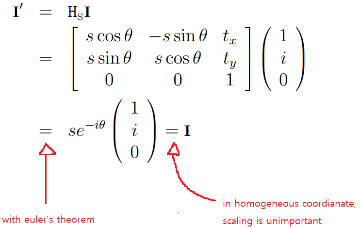
사영 왜곡된 이미지에서 원형점(the circular points) $I, J$ 를 식별하면 닮음 속성을 복원할 수 있습니다. 이는 원형점 $I, J$ 가 사영 변환 H에 고정된다는 것이 H가 닮음 변환인 것과 필요충분조건이기 때문입니다. 일반적으로 I와 J의 좌표는 아래와 같습니다.

$I = (\begin{matrix} 1 \\ i \\ 0 \end{matrix}), J = (\begin{matrix} 1 \\ - i \\ 0 \end{matrix}) .$

아래 그림은 circular points가 similarity transformation에 invariant 하다는 것을 보여줍니다.

figure2.7_6-2

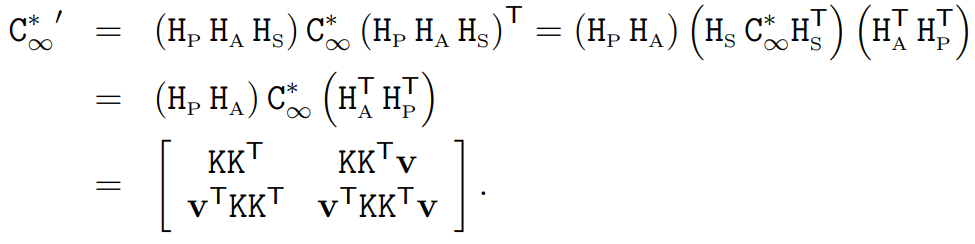
The conic dual to the circular points#

사영 왜곡된 이미지에서 circular points에 대한 dual conic $C_{\infty}^{*}$ 를 식별하여도 similarity 속성을 복원할 수 있습니다. 이는 $C_{\infty}^{*}$ 가 projective transformation H에 고정된다는 것이 H가 similarity transformation인 것과 필요충분조건이기 때문입니다.

figure2.7_7

※ circular points에 대한 duality conic $C_{\infty}^{*}$ 는 다음과 같이 주어집니다.

$C_{\infty}^{*} = I J^{T} + J I^{T}$

따라서 Conic $C_{\infty}^{*}$ 은 아래와 같이 표현할 수 있습니다.

$C_{\infty}^{*} = (\begin{matrix} 1 \\ i \\ 0 \end{matrix}) (\begin{matrix} 1 & - i & 0 \end{matrix}) + (\begin{matrix} 1 \\ - i \\ 0 \end{matrix}) (\begin{matrix} 1 & i & 0 \end{matrix}) = [\begin{matrix} 1 & 0 & 0 \\ 0 & 1 & 0 \\ 0 & 0 & 0 \end{matrix}]$

2.4.4 Angles on the projective plane#

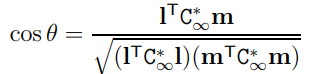
사영 평면에서 $C_{\infty}^{*}$ 을 결정하면 다음과 같은 방법으로 유클리드 각을 측정할 수 있습니다.

figure2.7_8

위 수식은 사영 변환에서 불변량이며, $l^{T} C_{\infty}^{*} m = 0$ 이면 직선 $l$ 과 $m$ 은 직교합니다.

2.4.5 Recovery of metric properties from images#

원형점을 표준 위치 $(1, \pm i, 0)^{T}$ 로 변환하면 사영 왜곡된 이미지에서 거리 속성을 복원할 수 있습니다. 그리고 Result 2.21.에 의해 실세상 평면과 복원된 이미지 사이의 변환이 닮음 변환임을 보일 수 있습니다.

**Metric Rectification using $C_{\infty}^{*}$** #

다음과 같이 $C_{\infty}^{*}$ 를 이용하여 사영 변환의 닮음 왜곡을 제외하고 사영과 아핀 구성 행렬을 모두 결정할 수 있습니다.

figure2.7_9

Metric rectification from affine distorted images#

이미지가 아핀 보정이 됐다고 가정하면, 거리 보정을 위해 원형점의 자유도 2를 결정하는 제약 조건 2개가 필요합니다. 실세상 평면에서 직각인 두 개의 이미지에서 제약 조건을 얻을 수 있습니다.

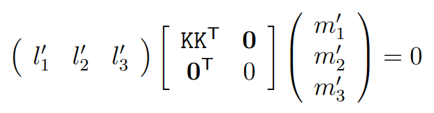
아핀 정정 이미지의 직선 $l^{'}, m^{'}$ 이 실세계에서 직교하는 선 $l, m$ 에 대응한다고 가정하면 $l^{' T} C_{\infty}^{*} m = 0, v = 0$ 을 이용할 수 있고, 바로 위에서 언급된 $C_{\infty}^{*}$ ’에 대한 공식을 다음과 같이 정리할 수 있습니다.

figure2.7_10

이것은 2 X 2 행렬 $S = K K^{T}$ 에 대한 선형 제약조건이다. 행렬 $S$ 는 대칭이므로 3개의 독립 원소를 가지며, scaling은 중요하지 않으므로 자유도는 2입니다.

따라서 두 선의 직교 조건은 $(l_{1}^{'} m_{1}^{'}, l_{1}^{'} m_{2}^{'} + l_{2}^{'} m_{1}^{'}, l_{2}^{'} m_{2}^{'}) s = 0$ 으로 표기할 수 있습니다. 이러한 방식으로 두 개의 직교하는 선 쌍에서 제약조건 두 개를 얻으면, Cholesky Decomposition을 이용하여 $K$ 를 구해낼 수 있고, $C_{\infty}^{*}$ ’를 계산할 수 있습니다.

아래 해당 코드를 첨부합니다.

img = cv2.imread('./figures/chessboard.jpg', cv2.IMREAD_COLOR)

# select two orthogonal pairs
st = [np.array([1157,  676]), np.array([989, 638]), np.array([1055,  544]), np.array([1221,  582])]
ed = [np.array([989, 638]), np.array([1055,  544]), np.array([1221,  582]), np.array([1157,  676])]
st = np.append(st, np.ones((4,1), dtype=np.int32), axis=1)
ed = np.append(ed, np.ones((4,1), dtype=np.int32), axis=1)

l1 = np.cross(st[0], ed[0])
l2 = np.cross(st[1], ed[1])

m1 = np.cross(st[2], ed[2])
m2 = np.cross(st[3], ed[3])

# constraints
ortho_constraint = np.array([[l1[0]*m1[0], l1[0]*m1[1]+l1[1]*m1[0], l1[1]*m1[1]],
                            [l2[0]*m2[0], l2[0]*m2[1]+l2[1]*m2[0], l2[1]*m2[1]]
                            ])

# decompose orthogonal constraint using SVD to gain S
U,S,V = np.linalg.svd(ortho_constraint, full_matrices=True)
S_matrix = np.diag(S)

# S = KK^T
# decompose S using Cholesky decomposition to gain K
K = np.linalg.cholesky(S_matrix)
K = K/K[1][1]

# Compute metric rectification matrix
H_m = np.eye(3)
H_m[:2,:2] = K
H_m = np.linalg.inv(H_m)

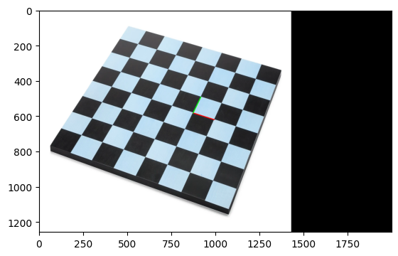
# recover the metric properties
dst = cv2.warpPerspective(img, H_m*H_A, (0,0))

cv2.line(img, st[0][:2], ed[0][:2], (255,0,0),3)
cv2.line(img, st[1][:2], ed[1][:2], (255,0,0),3)

cv2.line(img, st[2][:2], ed[2][:2], (0,0,255),3)
cv2.line(img, st[3][:2], ed[3][:2], (0,0,255),3)


concat = np.concatenate([img, dst], axis=1)
plt.imshow(concat)

<matplotlib.image.AxesImage at 0x169db0650>

../../_images/e8f79352e007367ee6eb6c88cec74fe1905e9e7735581d99701b625d9269e73d.png

Angle measurement code#

위 보정된 이미지에서 좌표를 찍어 측정해본 결과입니다.

st = [np.array([992, 621]), np.array([872, 583])]
ed = [np.array([872, 583]), np.array([916, 492])]
st = np.append(st, np.ones((2,1), dtype=np.int32), axis=1)
ed = np.append(ed, np.ones((2,1), dtype=np.int32), axis=1)

conic = np.array([[1,0,0],
                  [0,1,0],
                  [0,0,0]])

l = np.cross(st[0], ed[0])
l = l/l[2]
m = np.cross(st[1], ed[1])
m  = m/m[2]

# calulate the angle using conic
cos_theta = l.T@conic@m
val = np.sqrt((l.T@conic@l)*(m.T@conic@m))
cos_theta = cos_theta / val

theta = np.arccos(cos_theta) * 180 / np.pi
print('angle between l and m : ', theta)


cv2.line(dst, st[0][:2], ed[0][:2], (255,0,0),3)
cv2.line(dst, st[1][:2], ed[1][:2], (0,255,0),3)

plt.imshow(dst)

angle between l and m :  81.7667263783753

<matplotlib.image.AxesImage at 0x168e465d0>

../../_images/52176e834006f92730098ef202d608d410d325417b122abe4361ee30bb0c98c1.png

Metric rectification from original images#

아핀 왜곡된 이미지에서 거리 속성 복원한 위 사례와 유사하게, 원본 이미지에서 바로 거리 속성을 복원할 수 있습니다. 직선 $l$ 과 $m$ 을 실세상 평면에서 직교하는 직선의 이미지로 가정하면 $l^{' T} C_{\infty}^{*} m = 0$ 을 이용할 수 있고, 다음과 같이 $C_{\infty}^{*}$ 에 대한 선형 제약 조건을 얻습니다.

figure2.7_11

여기에서 $c = (a, b, c, d, e, f)^{T}$ 는 6차원 벡터로 표기한 $C_{\infty}^{*}$ 의 conic matrix 입니다. 이러한 제약조건 5개로 5 X 6 행렬을 만들면 $c$ 는 ( $C_{\infty}^{*}$ ) null vector가 됩니다. 따라서 $C_{\infty}^{*}$ 는 실세계에서 직교하는 다섯 선 쌍에서 선형적으로 결정할 수 있습니다.

Stratification#

$C_{\infty}^{*}$ 를 식별하여 원본 이미지에서 아핀 왜곡과 사영 왜곡을 한 번에 정정하는 방법을 배웠습니다. 그리고 사영 왜곡을 먼저 제거하고 아핀 왜곡을 제거하는 방법도 배웠습니다. 이러한 2단계 접근 방식을 Stratification 이라고 합니다. 비슷한 접근 방식을 3차원에서도 적용할 수 있습니다.

Reference#

Multiple view geometry in computer vision chapter 2.7