3. Data Preprocessing
![]()
In chapter 2, we explored the data in the Face Mask Detection dataset. In this chapter, we will perform data preprocessing.
Popular datasets have tens of thousands of images, but many datasets are created on a much smaller scale, raising the question of how to train a limited dataset.
You don’t have to find new images just because your dataset is limited. Instead, various images can be obtained using data augmentation.

Figure 3-1 Looks the same but is a different tennis ball (Source: https://nanonets.com/blog/data-augmentation-how-to-use-deep-learning-when-you-have-limited-data-part-2/ )
Figure 3-1 shows tennis balls that look identical to human eyes. However, the deep learning model sees all three tennis balls differently. With this principle, we can extract multiple data by modulating a single image.
In chapter 3.1, we will look at the torchvision.transforms and albumentations modules used for image augmentation. torchvision.transforms is a module officially provided by PyTorch, and albumentations is an optimized open source computer vision library, similar to OpenCV. It is a module that provides faster processing speed, along with other features.
Both modules can be used for augmentation when building an image classification model. However, the image augmentation function for building an object detection model is provided only by albumentations . Image augmentation for object detection should transform not only the image but also the bounding box, which is a function that torchvision.transforms does not provide.
Therefore, in chapter 3.2, we will practice bounding box augmentation using albumentations . Finally, in chapter 3.3, we will separate the data into training data and test data.
3.1. Augmentation Practice
For the augmentation practice, we will load the data using the code from chapter 2.1.
!git clone https://github.com/Pseudo-Lab/Tutorial-Book-Utils
!python Tutorial-Book-Utils/PL_data_loader.py --data FaceMaskDetection
!unzip -q Face\ Mask\ Detection.zip
Cloning into 'Tutorial-Book-Utils'...
remote: Enumerating objects: 12, done.
remote: Counting objects: 100% (12/12), done.
remote: Compressing objects: 100% (11/11), done.
remote: Total 12 (delta 1), reused 2 (delta 0), pack-reused 0
Unpacking objects: 100% (12/12), done.
Face Mask Detection.zip is done!
Make sure to use the latest version of the albumentations module by upgrading it if necessary. We can upgrade a specific module through the pip install --upgrade command.
!pip install --upgrade albumentations
To visualize the augmentation output, let’s use the bounding box schematic code from chapter 2.3.
import os
import glob
import matplotlib.pyplot as plt
import matplotlib.patches as patches
from bs4 import BeautifulSoup

def generate_box(obj):

    xmin = float(obj.find('xmin').text)
    ymin = float(obj.find('ymin').text)
    xmax = float(obj.find('xmax').text)
    ymax = float(obj.find('ymax').text)

    return [xmin, ymin, xmax, ymax]

def generate_label(obj):

    if obj.find('name').text == "with_mask":

        return 1

    elif obj.find('name').text == "mask_weared_incorrect":

        return 2

    return 0


def generate_target(file):
    with open(file) as f:
        data = f.read()
        soup = BeautifulSoup(data, "html.parser")
        objects = soup.find_all("object")

        num_objs = len(objects)

        boxes = []
        labels = []
        for i in objects:
            boxes.append(generate_box(i))
            labels.append(generate_label(i))

        boxes = torch.as_tensor(boxes, dtype=torch.float32)
        labels = torch.as_tensor(labels, dtype=torch.int64)

        target = {}
        target["boxes"] = boxes
        target["labels"] = labels

        return target

def plot_image_from_output(img, annotation):

    img = img.permute(1,2,0)

    fig,ax = plt.subplots(1)
    ax.imshow(img)

    for idx in range(len(annotation["boxes"])):
        xmin, ymin, xmax, ymax = annotation["boxes"][idx]

        if annotation['labels'][idx] == 0 :
            rect = patches.Rectangle((xmin,ymin),(xmax-xmin),(ymax-ymin),linewidth=1,edgecolor='r',facecolor='none')

        elif annotation['labels'][idx] == 1 :

            rect = patches.Rectangle((xmin,ymin),(xmax-xmin),(ymax-ymin),linewidth=1,edgecolor='g',facecolor='none')

        else :

            rect = patches.Rectangle((xmin,ymin),(xmax-xmin),(ymax-ymin),linewidth=1,edgecolor='orange',facecolor='none')

        ax.add_patch(rect)

    plt.show()
There are some differences from the functions used in chapter 2. We can see that the torch.as_tensor function has been added to the generate_target function to prepare for the operation between tensors when training the deep learning model later.
Additionally, the plot_image function introduced in chapter 2 read images from a file path. Now, the plot_image_from_output function visualizes the image after it has been converted to torch.Tensor . In PyTorch, images are expressed as [channels, height, width] , whereas in matplotlib they are expressed as [height, width, channels] . Therefore, we must use the permute function to change the channel order expected by matplotlib .
3.1.1. Torchvision Transforms
To practice torchvision.transforms, let’s first define the TorchvisionDataset class. The TorchvisionDataset class loads the image through the __getitem__ method and then proceeds with data augmentation. Augmentation is performed according to the rule stored in the transform parameter. To measure time, it uses the time function, and finally returns image , label , and total_time .
from PIL import Image
import cv2
import numpy as np
import time
import torch
import torchvision
from torch.utils.data import Dataset
from torchvision import transforms
import albumentations
import albumentations.pytorch
from matplotlib import pyplot as plt
import os
import random

class TorchvisionMaskDataset(Dataset):
    def __init__(self, path, transform=None):
        self.path = path
        self.imgs = list(sorted(os.listdir(self.path)))
        self.transform = transform

    def __len__(self):
        return len(self.imgs)

    def __getitem__(self, idx):
        file_image = self.imgs[idx]
        file_label = self.imgs[idx][:-3] + 'xml'
        img_path = os.path.join(self.path, file_image)

        if 'test' in self.path:
            label_path = os.path.join("test_annotations/", file_label)
        else:
            label_path = os.path.join("annotations/", file_label)

        img = Image.open(img_path).convert("RGB")

        target = generate_target(label_path)

        start_t = time.time()
        if self.transform:
            img = self.transform(img)

        total_time = (time.time() - start_t)

        return img, target, total_time
Let’s practice image augmentation using the function provided in torchvision.transforms. After setting the image size (300, 300), we will crop it to size 224. Then we’ll randomly change the image’s brightness, contrast, saturation, and hue. Finally, after inverting the image horizontally, we will convert it to a tensor.
torchvision_transform = transforms.Compose([
    transforms.Resize((300, 300)),
    transforms.RandomCrop(224),
    transforms.ColorJitter(brightness=0.2, contrast=0.2, saturation=0.2, hue=0.2),
    transforms.RandomHorizontalFlip(p = 1),
    transforms.ToTensor(),
])

torchvision_dataset = TorchvisionMaskDataset(
    path = 'images/',
    transform = torchvision_transform
)
We can resize the image through the Resize function, then we can crop the image through the RandomCrop function provided by transforms. The ColorJitter function randomly changes the brightness, contrast, saturation, and hue. The RandomHorizontalFlip performs a horizontal inversion with a defined probability of p. Let’s run the code below to compare the image before and after the change.
only_totensor = transforms.Compose([transforms.ToTensor()])
torchvision_dataset_no_transform = TorchvisionMaskDataset(
path = 'images/',
transform = only_totensor
)
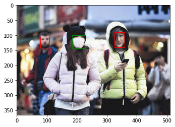
img, annot, transform_time = torchvision_dataset_no_transform[0]
print('Before applying transforms')
plot_image_from_output(img, annot)
Before applying transforms
img, annot, transform_time = torchvision_dataset[0]

print('After applying transforms')
plot_image_from_output(img, annot)
After applying transforms
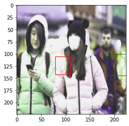
We can see that the mentioned changes have been applied to the image. However, while the image itself has changed, the bounding box has not. We can see that the augmentation provided by torchvision.transform only affects the image value, not the location of the bounding box.
For image classification, the label value is fixed even if the image changes. But for object detection, the label value will also change as the image changes. We’ll see how to solve this problem in chapter 3.2. First, however, we will continue to compare the torchvision and albumentations modules. We will calculate the time spent converting the image in torchvision_dataset and measure the time it will take to repeat it 100 times using the code below.
total_time = 0
for i in range(100):
  sample, _, transform_time = torchvision_dataset[0]
  total_time += transform_time

print("torchvision time: {} ms".format(total_time*10))
torchvision time: 10.138509273529053 ms
It took about 10 to 12 ms to perform the image conversion 100 times. In the next section, we will check the augmentation speed of the albumentations module.
3.1.2. Albumentations
In chapter 3.1.1, we measured the conversion speed of torchvision.transforms. In this section, we will look at another augmentation module, albumentations. Like we did for torchvision, let’s first define the dataset class. AlbumentationDataset has a similar structure to TorchVisionDataset. It reads the image using the cv2 module and converts it to RGB. After converting the image, the result is returned.
class AlbumentationsDataset(Dataset):
    def __init__(self, path, transform=None):
        self.path = path
        self.imgs = list(sorted(os.listdir(self.path)))
        self.transform = transform

    def __len__(self):
        return len(self.imgs)

    def __getitem__(self, idx):
        file_image = self.imgs[idx]
        file_label = self.imgs[idx][:-3] + 'xml'
        img_path = os.path.join(self.path, file_image)

        if 'test' in self.path:
            label_path = os.path.join("test_annotations/", file_label)
        else:
            label_path = os.path.join("annotations/", file_label)

        # Read an image with OpenCV
        image = cv2.imread(img_path)
        image = cv2.cvtColor(image, cv2.COLOR_BGR2RGB)

        target = generate_target(label_path)

        start_t = time.time()
        if self.transform:
            augmented = self.transform(image=image)
            total_time = (time.time() - start_t)
            image = augmented['image']


        return image, target, total_time
For a speed comparison with torchvision.transform, let’s use the same functions: Resize, RandomCrop, ColorJitter, and HorizontalFlip. Then we will compare the images before and after the change.
# Same transform with torchvision_transform
albumentations_transform = albumentations.Compose([
    albumentations.Resize(300, 300),
    albumentations.RandomCrop(224, 224),
    albumentations.ColorJitter(p=1),
    albumentations.HorizontalFlip(p=1),
    albumentations.pytorch.transforms.ToTensor()
])
# Before applying transforms
img, annot, transform_time = torchvision_dataset_no_transform[0]
plot_image_from_output(img, annot)

# After applying transforms
albumentation_dataset = AlbumentationsDataset(
    path = 'images/',
    transform = albumentations_transform
)

img, annot, transform_time = albumentation_dataset[0]
plot_image_from_output(img, annot)
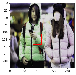
Like torchvision.transform, the image has been transformed, but the bounding box has not changed. To measure the speed, we will apply albumentation 100 times.
total_time = 0
for i in range(100):
    sample, _, transform_time = albumentation_dataset[0]
    total_time += transform_time

print("albumentations time/sample: {} ms".format(total_time*10))
albumentations time/sample: 2.1135759353637695 ms
It took about 2.0 to 2.5 ms to perform the image conversion 100 times. Compared to torchvision.transforms, it is about 4 times faster.
3.1.3. Probability-Based Augmentation Combination
Albmentations is not only faster than torchvision.transforms, but also provides a new function. In this section, we will look at the OneOf function provided by Albumentations. This function retrieves the augmentation functions in the list based on a given probability value. The probability value of the list and of the corresponding function are considered together to decide whether or not to execute. The OneOf functions below each have a probability of being selected. Since the 3 albumentations functions inside each function are also given a probability value of 1, we can see that one of the 3 functions is selected and executed with an actual probability of 1/3. There are various possible augmentations that can be created by adjusting the probability value in this way.
albumentations_transform_oneof = albumentations.Compose([
    albumentations.Resize(300, 300),
    albumentations.RandomCrop(224, 224),
    albumentations.OneOf([
                          albumentations.HorizontalFlip(p=1),
                          albumentations.RandomRotate90(p=1),
                          albumentations.VerticalFlip(p=1)
    ], p=1),
    albumentations.OneOf([
                          albumentations.MotionBlur(p=1),
                          albumentations.OpticalDistortion(p=1),
                          albumentations.GaussNoise(p=1)
    ], p=1),
    albumentations.pytorch.ToTensor()
])
Below is the result of applying albumentations_transform_oneof to an image 10 times.
albumentation_dataset_oneof = AlbumentationsDataset(
    path = 'images/',
    transform = albumentations_transform_oneof
)

num_samples = 10
fig, ax = plt.subplots(1, num_samples, figsize=(25, 5))
for i in range(num_samples):
  ax[i].imshow(transforms.ToPILImage()(albumentation_dataset_oneof[0][0]))
  ax[i].axis('off')

3.2. Bounding Box Augmentation
When performing augmentation on the image used to build the object detection model, the bounding box conversion must be carried out along with the image conversion. As we saw in chapter 3.1, if the bounding box is not converted together, the model training will not work properly because the bounding box is detecting the wrong place. Bounding box augmentation is possible by using the bbox_params parameter in the Compose function provided by Albumentations.
First, let’s create a new dataset class using the code below. The transform part of the AlbumentationsDataset class in section 3.1.2 has been modified. Not only the image but also the bounding box is being transformed, so the necessary input and output values are modified.
class BboxAugmentationDataset(Dataset):
    def __init__(self, path, transform=None):
        self.path = path
        self.imgs = list(sorted(os.listdir(self.path)))
        self.transform = transform

    def __len__(self):
        return len(self.imgs)

    def __getitem__(self, idx):
        file_image = self.imgs[idx]
        file_label = self.imgs[idx][:-3] + 'xml'
        img_path = os.path.join(self.path, file_image)

        if 'test' in self.path:
            label_path = os.path.join("test_annotations/", file_label)
        else:
            label_path = os.path.join("annotations/", file_label)

        image = cv2.imread(img_path)
        image = cv2.cvtColor(image, cv2.COLOR_BGR2RGB)

        target = generate_target(label_path)

        if self.transform:
            transformed = self.transform(image = image, bboxes = target['boxes'], labels = target['labels'])
            image = transformed['image']
            target = {'boxes':transformed['bboxes'], 'labels':transformed['labels']}


        return image, target
Next, let’s use the albumentations.Compose function to define the transformation. The first thing we will do is perform a horizontal flip, then we will rotate between -90 and 90 degrees. Enter the albumentations.BboxParams object into the bbox_params parameter in order to convert the bounding box as well. In the Face Mask Detection dataset, the bounding box notation is xmin , ymin , xmax , ymax , which is the same as pascal_voc notation. Therefore, enter pascal_voc in the format parameter. Also, enter labels in label_field to store the class values for each object in the labels parameter when transform is performed.
bbox_transform = albumentations.Compose(
    [albumentations.HorizontalFlip(p=1),
     albumentations.Rotate(p=1),
     albumentations.pytorch.transforms.ToTensor()],
    bbox_params=albumentations.BboxParams(format='pascal_voc', label_fields=['labels']),
)
Now let’s activate the BboxAugmentationDataset class and check the augmentation result.
bbox_transform_dataset = BboxAugmentationDataset(
    path = 'images/',
    transform = bbox_transform
)

img, annot = bbox_transform_dataset[0]
plot_image_from_output(img, annot)
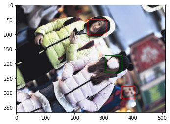
Whenever we run the code above, the image is converted and output. In addition to that, the bounding box is also properly transformed so we can see that it accurately detects masked faces in the transformed image. We will build a model in chapters 4 and 5 using the data created by converting the image and bounding box together.
3.3. Data Separation
To build an Artificial Intelligence model, we need training data and test data. The training data is used when training the model, and the test data is used when evaluating the model. Test data must not overlap with training data. Let’s divide the data imported in chapter 3.1 into training data and test data. First, let’s check the total number of data with the code below.
print(len(os.listdir('annotations')))
print(len(os.listdir('images')))
853
853
We can see that there are a total of 853 images. Usually, the ratio of training data to test data is 7:3. This data has a small total compared to more comprehensive datasets, so let’s take an 8:2 ratio. In order to use 170 of the 853 data as test data, we will move the data to a separate folder. First, create a folder to contain test data using the Linux command mkdir.
!mkdir test_images
!mkdir test_annotations
If we run the code above, the test_images folder and test_annotations folder will be created. Now, we will move 170 files each from the images folder and annotations folder into the newly created folders. We will use the sample function in the random module to randomly extract numbers and use them as index values.
import random
random.seed(1234)
idx = random.sample(range(853), 170)
print(len(idx))
print(idx[:10])
170
[796, 451, 119, 7, 92, 826, 596, 35, 687, 709]
import numpy as np
import shutil

for img in np.array(sorted(os.listdir('images')))[idx]:
    shutil.move('images/'+img, 'test_images/'+img)

for annot in np.array(sorted(os.listdir('annotations')))[idx]:
    shutil.move('annotations/'+annot, 'test_annotations/'+annot)
As seen in the code above, we can use the shutil package to move 170 images and 170 annotation files to the test_images folder and test_annotations folder, respectively. Let’s check the number of files in each folder.
print(len(os.listdir('annotations')))
print(len(os.listdir('images')))
print(len(os.listdir('test_annotations')))
print(len(os.listdir('test_images')))
683
683
170
170
For image classification, you only need to check the number of images after dividing the dataset. But for object detection, it is necessary to check how many objects for each class exist in the dataset. Let’s use the code below to check the number of objects by class in the dataset.
from tqdm import tqdm
import pandas as pd
from collections import Counter

def get_num_objects_for_each_class(dataset):

    total_labels = []

    for img, annot in tqdm(dataset, position = 0, leave = True):
        total_labels += [int(i) for i in annot['labels']]

    return Counter(total_labels)


train_data =  BboxAugmentationDataset(
    path = 'images/'
)

test_data =  BboxAugmentationDataset(
    path = 'test_images/'
)

train_objects = get_num_objects_for_each_class(train_data)
test_objects = get_num_objects_for_each_class(test_data)

print('\n Object in training data', train_objects)
print('\n Object in test data', test_objects)
100%|██████████| 683/683 [00:13<00:00, 51.22it/s]
100%|██████████| 170/170 [00:03<00:00, 52.67it/s]
Object in training data Counter({1: 2691, 0: 532, 2: 97})

Object in test data Counter({1: 541, 0: 185, 2: 26})
ㅤ
get_num_objects_for_each_class is a function that stores the label values of all bounding boxes in the dataset in total_labels and then uses the Counter class to count and return the number of each label. In the training data, there are 532 objects in class 0, 2,691 objects in class 1, and 97 objects in class 2. In the test data, there are 185 objects in class 0, 541 objects in class 1, and 26 objects in class 2. We can confirm that the data is divided appropriately by seeing that the ratio of 0,1,2 is similar for each dataset.
So far, we have seen how to use the Albumentations module to inflate the number of images used to build an object detection model, and we have seen how to separate the owned data into training data and test data. In chapter 4, we will build a mask wearing detection model by training RetinaNet, a one-stage model.