1. Introduction to Object Detection
![]()
Object Detection is a field of computer vision technology in which objects of interest within a given image are detected.
If an artificial intelligence model determines that the image on the left in Figure 1-1 is of a dog, the model is an image classification model. However, if the artificial intelligence model classifies the object as a dog while also detecting the location of the object, as shown in the picture on the right, the model is an object detection model.

Figure 1-1 Comparison of image classification model and object detection model (Source: https://www.pexels.com/search/dog/)
The object detection model can be used in many fields. The most representative case is in an autonomous vehicle. In order to create an autonomous vehicle, computers must be able to recognize surrounding objects by themselves. For instance, the computer should recognize traffic signals; when there is a red light, the vehicle should know to stop.
Object detection technology is also used for efficient resource management in the field of security. In general, CCTVs record continuously, so a huge amount of memory is required. However, in combination with object detection technology, memory can be used efficiently by starting a recording only when a specific object is detected.
In this chapter, we will build an object detection model that detects masks. The model we built detects the position of the face in a given image and checks if the face is masked.
1.1. Bounding Box
Before creating an object detection model, the first step is to create a bounding box. Since the amount of data used in the object detection model is vast, the object can be correctly detected through a bounding box. In the deep learning process, only the bounding box area is targeted, so we can train efficiently.
The bounding box is a method that helps us train a model efficiently by detecting specific objects. In the object detection model, bounding boxes are used to specify the target location. The target position is expressed as a rectangle using the X and Y axes. The bounding box value is expressed as (X min, Y min, X max, Y max).

Figure 1-2 Bounding box area specified as pixel value (Source: https://github.com/sgrvinod/a-PyTorch-Tutorial-to-Object-Detection)
As shown in Figure 1-2, the area between the minimum and maximum X and Y values is set as the bounding box area. However, the X and Y values in Figure 1-2 are pixel values and should be converted into a value between 0 and 1 for efficient calculation.

Figure 1-3 Bounding box area specified in percentiles (Source: https://github.com/sgrvinod/a-PyTorch-Tutorial-to-Object-Detection/raw/master/img/bc2.PNG)
The X and Y values in Figure 1-3 are calculated by dividing the original pixel X- and Y-values of the bounding box by the maximum pixel X-value of 971 and the maximum pixel Y-value of 547, respectively. For example, the bounding box minimum X-value of 640 is divided by 971 to get 0.66. This normalization can be seen as a process for efficient computation, but it is not essential.
Depending on the dataset, the bounding box value may be included as metadata. If there is no metadata, the bounding box can be specified through separate code implementation. The Face Mask Detection dataset used in this tutorial provides bounding boxes. We will diagram the bounding box in chapter 2.
1.2. Model Type
The object detection model can be largely divided into one-stage and two-stage models. Let’s take a look at each model type.

Figure 1-4 Object detection algorithm timeline (Source: Zou et al. 2019. Object Detection in 20 Years: A Survey)
Figure 1-4 shows the genealogy of the object detection model. Object detection models based on deep learning appeared in 2012 and can be divided into one-stage detectors and two-stage detectors. To understand the two types of flows, we need to understand the concepts of classification and region proposal. Classification is to classify an object, and region proposal is an algorithm that finds an area where an object is likely to be.
Two-stage detectors perform well in terms of object detection accuracy, but are limited to real-time detection due to their slow prediction speed. To solve this speed problem, one-stage detectors, which simultaneously perform classification and region proposition, have been created. In the next section, we will examine the structure of one-stage and two-stage detectors.
1.2.1. One-Stage Detector
One-stage detection is a method of obtaining results by performing classification and regional proposal simultaneously. After inputting the image into the model, image features are extracted using the Conv Layer as shown in Figure 1-5.

Figure 1-5 One-Stage Detector Structure (Source: https://jdselectron.tistory.com/101)
1.2.2. Two-Stage Detector
Two-stage detection is a method of obtaining results by sequentially performing classification and regional proposal. As shown in Figure 1-6, we can see that region proposal and classification are executed sequentially.

Figure 1-6 Two-Stage Detector structure (source: https://jdselectron.tistory.com/101)
As a result, one-stage detection is relatively fast but has low accuracy, and two-stage detection is relatively slow but has higher accuracy.
1.3. Model Structure
There are several structures for each one-stage and two-stage detector. R-CNN, Fast R-CNN, and Faster R-CNN are two-stage detectors, while YOLO, SSD, and RetinaNet are one-stage detectors. Let’s look at the characteristics of each model structure.
1.3.1. R-CNN

Figure 1-8 R-CNN structure (Source: Girshick et al. 2014. Rich feature gierarchies for accurate object detection and semantic segmentation)
R-CNN creates a region proposal for an image using Selective Search. Each created candidate region is wrapped in a fixed size by force and used as an input to the CNN. The feature map from the CNN is classified through SVM and the bounding-box is adjusted through Regressor. It has the disadvantage that it requires a large amount of storage space and is slow, since the image must be transformed or lost by wrapping and the CNN must be rotated as many times as the number of candidate regions.
1.3.2. Fast R-CNN
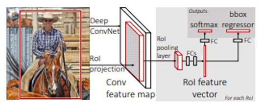
Figure 1-9 Fast R-CNN structure (Source: Girshick. ICCV 2015. Fast R-CNN)
Unlike R-CNNs, which apply a CNN to each candidate region, in a Fast R-CNN structure, a candidate region is created from the feature map generated by applying a CNN to the entire image. The generated candidate region is extracted as a fixed size feature vector through RoI pooling. After passing through the FC layer on the feature vector, classify it through Softmax, and adjust the bounding-box through Regressor.
1.3.3. Faster R-CNN


Figure 1-10 Faster R-CNN Structure (Source: Ren et al. 2016. Faster R-CNN: Towards Real-Time Object Detection with Region Proposal Networks)
Faster R-CNNs use a Region Proposal Network (RPN), which uses deep learning in place of the Selective Search step. RPNs predict the candidate region with an anchor-box at each point taken by the sliding-window when calculating the CNN in the feature map. The anchor box is a bounding box with several preset ratios and sizes. The candidate regions obtained from the RPN are sorted in the order of IoU, and the final candidate regions are selected through the Non-Maximum Suppression (NMS) algorithm. To fix the size of the selected candidate region, RoI pooling is performed, and then the process proceeds in the same manner as a Fast R-CNN.
1.3.4. YOLO

Figure 1-11 YOLO structure (Source: Redmon et al. 2016. You Only Look Once: Unified, Real-Time Object Detection)
Treating the bounding-box and class probability as a single problem, the YOLO structure predicts the class and location of an object at the same time. In order to use it, we divide the image into grids of a certain size to predict the bounding box for each grid. We will train the model with the confidence score values for the bounding boxes and the class score values for the grid cells. It is a very fast and simple process, but it is relatively inaccurate for small objects.
1.3.5. SSD

Figure 1-12 SSD structure (Source: Liu et al. 2016. SSD: Single Shot MultiBox Detector)
The SSD calculates the bounding box’s class score and offset (position coordinates) for each feature map that appears after each Convolutional Layer. The final bounding box is determined through the NMS algorithm. This has the advantage of being able to detect both small and large objects, since each feature map has a different scale.
1.3.6. RetinaNet

Figure 1-13 Focal Loss (Source: Lin et al. 2018. Focal Loss for Dense Object Detection)
RetinaNet improves upon the low performance of existing One-Stage Detectors by changing the loss function calculated during model training. One-Stage Detector trains itself by suggesting up to 100,000 candidates during the training phase. Most of them are classified as background classes and only 10 or less candidates are actually detecting the objects of interest. By reducing the loss value for relatively easy to classify background candidates, the weights of the loss of real objects that are difficult to classify are increased. Accordingly, we focus on training about objects of interest. RetinaNet is fast and performs similarly to a two-stage detector.